
- Tours/Car Rental
- D’ Lucky Garden Inn & Resorts


Underground River (Day Tours)

Firefly Watching (Night Tours)

Honda Bay Tour (Day Tours)

Palawan City Tour (Day Tours)

DOT Quality Seal of Excellence

We offer a full spectrum of tour packages in Palawan and international tours.We have competitively priced group tours and you can also request for a fully customized private tours.Our mission is to design affordable top quality tours at a competitive low prices while enhancing the enjoyment for people visiting each destinations with high quality of service for our customers.
Puerto Princesa City Island Package
Puerto Princesa Underground River Day Tour Package
Day tour to Honda bay
Travel 2 cities Puerto & El Nido 5d4n
Economy 4d3n Puerto Princesa Adventure Package
- ↘ Featured Travel
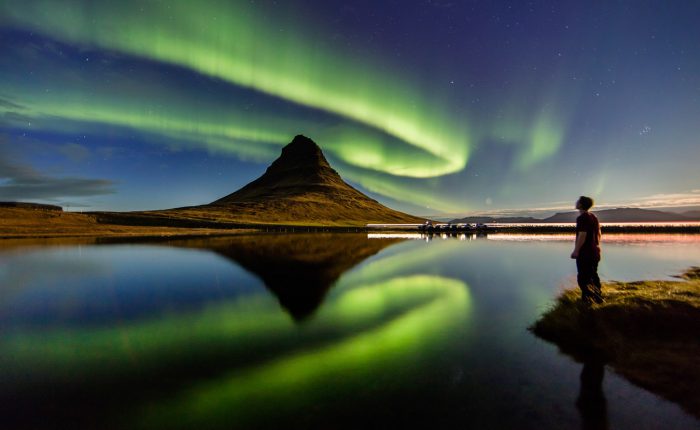
- Puerto Princesa’s pride is easily the Puerto Princesa Subterranean River (or Underground River), a UNESCO World Heritage Site and one of the New 7 Wonders of Nature. The 8.2-kilometer river, said to be the longest navigable underground river in the world... More »


Tours and Trip packages, Globally
Search, compare and book 15,000+ multiday tours all over the world.
Customize your trip with an Expert Trip Designer
Book your trip when it is perfectly designed and customized, just for you.
- Customized Tours
A strict screening process ensures that we only offer the best tours and trip packages globally.
We guarantee you the best price. Found a lower price? We will match it. Learn more
We CO 2 offset all tour bookings via investments in carbon reduction projects. Learn more
Customers have rated our trips 4.8 of 5 stars out of more than 25,000 trip ratings.
Top Destinations
Our top destinations. See them by continent.
Top Deals Worldwide
The best tours and trip deals, globally.

Featured Trips
Popular tours and trip packages. View them by travel style.

Mexico Highlights (from Cancun) Express Travel Pass

Langtang Trek with Chopper Return

Premium Spain in Depth

Jewels of France including Normandy

Best of Holland

Cocktail History Tour

Explore Croatia
Customize your trip with an expert trip designer.

Latest Travel Guides
View our travel guides giving you travel insights, ideas, and tips across the world.

Sweden in October: Weather, Mushroom Picking and More!
October in Sweden experiences the peak of fall season as the landscape bursts with fiery colors across the southern and central re ...Read more

One Week in Canada: Top 3 Recommendations
Experience Canada’s beauty in just one week with our carefully curated itineraries! Canada has a range of experiences for al ...Read more

South Korea in April: Weather, Cycling and More!
White and pink pastel cherry blossoms take over South Korea in April, making it one of the most sought-after months to visit. It i ...Read more

South Korea in January: Weather, Winter Sports and More!
January is the coldest month and the low travel season in South Korea. Just make sure to wrap up warm, and you can see the top sit ...Read more

China in March: Weather, Tips and More
Beautiful architecture at West Lake in Hangzhou in China in March.Though the weather in China in March is still chilly in places, ...Read more

2 Weeks in Canada: Top 3 Itinerary Recommendations
Canada is a vast country, and exploring its entirety on a single trip is practically impossible. So, it is best to pick one or two ...Read more

South Korea in March: Weather, Cherry Blossoms and More!
March in South Korea marks the transition from winter to spring, offering an ideal blend of pleasant weather, picturesque landscap ...Read more
- Italy Tours
- France Tours
- Spain Tours
- Portugal Tours
- Hungary Tours
- Holland Tours
- Croatia Tours
- England Tours
- Greece Tours
- Turkey Tours
- Vietnam Tours
- Nepal Tours
- India Tours
- Thailand Tours
- China Tours
- Combodia Tours
- Indonesia Tours
- Japan Tours
- South Korea Tours
- Sri Lanka Tours
North America
- Costa Rica Tours
- Mexico Tours
- Canada Tours
- Panama Tours
- Nicaragua Tours
- Belize Tours
South America
- Argentina Tours
- Chile Tours
- Brazil Tours
- Ecuador Tours
- Bolivia Tours
- Colombia Tours
- Tanzania Tours
- Kenya Tours
- South Africa Tours
- Egypt Tours
- Morocco Tours
- Zimbabwe Tours
- Uganda Tours
- Zambia Tours
- Namibia Tours
- Rwanda Tours
- Australia Tours
- New Zealand Tours
- Papua New Guinea Tours
Central America
- Guatemala Tours
- El Salvador Tours
East Africa
- Ethiopia Tours
- Madagascar Tours
- Seychelles Tours
- Sudan Tours
Northern Europe
- Iceland Tours
- Norway Tours
- Denmark Tours
- Finland Tours
- Sweden Tours
Middle East
- Jordan Tours
- Israel Tours
- Romania Tours
- Albania Tours
- Serbia Tours
- Montenegro Tours
- Bulgaria Tours
- Antarctica Tours
- Greenland Tours

Around the World Tours & Travel Packages 2024/2025
16 around the world trips. compare tour itineraries from 17 tour companies. 7 reviews. 5/5 avg rating., popular around the world tours.

Road to Paris

Road Scholar World Academy Segment 1: Indian Ocean to Cape Town
- Discover the incredible biodiversity of Madagascar at a protected reserve home to colorful birds, reptiles and lemurs.
- Explore St. Lucia National Park, where a sunset boat safari gives you the chance to see hippos and Nile crocodiles up close.
- Take a cable car to the top of Table Mountain for incredible views of Cape Town.

Dream Journey Around the World
- Visiting the Plaza de Armas with the beautiful buildings of the government Palace
- View the Belvedere Palace, Prater Amusement Park, the UN buildings, St. Stephen's Cathedral
- See Vajdahunyad castle, Széchenyi Spa, the Opera, the Synagogue of Dohány Street, St. Stephen’s Basilica and the decorative Parliament building.
- Visit the Great Sphinx of Giza and the Great Pyramids*
- Visit the Karnak Temple Complex and the Temple of Luxor on the East side of the Nile.

New York To New York
- Step into the Monte Carlo-inspired Empire Casino which offers a full variety of opportunities to tempt Lady Luck.
- Travel back to the grand old days of Venice at one of our Masquerade balls. Every evening on board is a real event and attending one of our balls in the Queens Room means you're in for a truly special evening.
- The quality and range of literature available in this beautiful room magnifies the stunning views over the bow. Take the time to linger over more than 8,000 books, in the largest library at sea.
- Wake yourself up with a brisk walk or breezy jog around our promenade deck. Three laps make a mile!
- Barossa Valley is famous worldwide for producing some wonderful boutique wines and internationally recognised names.

Oregon to India Rafting & Trekking
- This is a outdoor leadership course designed for age range 18 - 25
- Build core skills: Learn and practice wilderness, teamwork and leadership skills. Form a crew that supports and encourages one another, and in the thick of challenges, discover there is more in you than you know.
- Practice Outward Bound values: Learn to incorporate Outward Bound values into everyday life by pushing your own limits and seeking challenge as an opportunity for personal growth.
- Demonstrate mastery: As the course nears the end, take on more leadership and decision-making responsibilities. Work together to apply new skills and achieve team goals during this final phase of the expedition.
- What you’ll learn: Return home a stronger, more resilient individual. Discover increased self-confidence, improved leadership, and a desire to make a difference.

Scandinavian Capitals & Fjords 10-day
- Explore Stockholm Old Town Sightseeing Tour
- Discover Oslo - the fabulous capital of Norway.
- Visiting Frogner Park in Oslo
- Floibanen funicular ride in Bergen
- Fjords boat trip from Flam to Bergen

Road Scholar World Academy Semester 2: West from Asia to Europe
- Experience an unforgettable voyage from Singapore to England along the famed Suez Canal route.
- Explore wonders including the temples of Bali, the rock-cut city of Petra and Pompeii.
- For the first time, Road Scholar World Academy takes place aboard Holland America Line’s elegant ms Rotterdam.

San Francisco to Hong Kong
- Visit the Museum of Modern Art or head for the celebrated vineyards of the Napa and Sonoma Valleys.
- Experience Honolulu from a totally different angle on this thrilling helicopter ride.
- Explore the sea whilst whale watching aboard the high-tech, twin hulled 140 foot Navatek.
- Experience the thrill of swimming with sharks and schools of colourful tropical fish followed by a picnic on the beach.
- Experience the underwater wonders of Bora Bora's picturesque Lagoon by underwater scooter.
All Around the World , expedition cruises, self guided adventures and vacation packages. Find the best guided and expert planned vacation and holiday packages. Read more about Around the World

Small Group Around the World Tours
Best Around the World Tours by Duration
Tours, Cruises & Private Trips
Best Around the World Tours by Price
Top Around the World Attractions & Experiences
Top Around the World Experiences
Diverse experiences on around the world tour .
- Meeting locals from several different countries and discovering wonderful similarities and differences
- Seeing whales breach from the balcony of your cruise stateroom and diving and snorkeling in vibrant coral reefs like the Great Barrier reef
- Enjoying local cuisines, exploring street food markets, and taking cooking classes to learn how to make traditional national dishes
- Wandering around many archaeological ruins and historical sites like Machu Picchu , pyramids of Giza , and the historical city of Petra
- Discovering unique cultures and taking part in traditional festivals or ceremonies like Holi or Día de Muertos
- Hiking among different landscapes, encountering majestic wildlife on African Safaris , and taking memorable pictures
- Making lifelong friends from around the world
- Indulging in luxury around the world trips featuring traditional Japanese ryokan, floating hotels in the Maldives, or ice hotels in Sweden for a unique experience.
- Visiting all the most famous locations during a single trip with custom-planned tours around the world — No need to pick and choose!
Around the World Tours & Travel Guide
Around the World Attractions & Landmarks Guide
World travel is truly one of the most unforgettable experiences. As you visit multiple countries and continents, you gain a deep understanding of hundreds of cultures and forge wonderful connections with people around the world.
A small ship or 'expedition' cruise is one of the most popular modes of travel for a trip around the world. Many young people opt for overland tours to see the world because of budget and the community style. They usually use a few different modes of travel like trains or buses or join small group tours to individual destinations.
You can also design a custom round-the-world trip to suit your preferences for price, duration, accommodation, and more. Choose the countries you wish to visit and super-personalize your world tour for the activities you enjoy.
Luxury Around the World Trips
Imagine waking up in lavish four or five-star accommodations, imbibed with unmatched comfort and elegance. Think boutique lodges nestled in scenic landscapes to high-end homestays steeped in local charm!
That's the essence of our exclusively curated around-the-world luxury tours. Choose one of our private guided world tours to explore iconic landmarks, access hidden gems, and indulge in gastronomic experiences redefining culinary pleasure.
Raise the bar for your travel experience—personalize your world trip and enjoy unparalleled service at every stop tailored to your preferences.
How Long Should You Go For?
A round-the-world trip typically takes longer than a week or two. Your world tour should not be much shorter than one month.
With one month to go around the world, you'll probably stick to one broad region. Long trips are a great way to really learn the nuances and extensiveness of human and geological history and how pronounced they can be in a relatively small area. You'll also gain a unique insight into fascinating cultural similarities and differences.
Most trips around the world are a bit longer than one month, typically between two and four months. The number of countries and continents you'll visit on your world tour can vary quite a bit, mainly based on how you get from place to place and the length of excursion allotted for by the itinerary.
How Much Does a Trip Around the World Cost?
One of the benefits of traveling on a package tour around the world is the cost-cutting aspect. Typically, some of your meals will be covered, along with a good amount of transportation and almost all accommodations (this is an excellent reason to book a small ship cruise).
In addition, your tour will have many activities planned to explore the culture and history of each destination, as well as enjoy the natural beauty with hikes and other exciting outdoor ventures. These activities are not always included in the price, which can be a good thing as it allows you to join as many or as few activities as you'd like, depending on your preferences.
Typically, airfare to and from the start city and ending city to your final destination is not included in the tour price, but after that, you can expect to save a lot in expenses.
Note that you'll be around the same group of people for a very extended period, and your ability to be flexible in each destination will be limited. If you want to stay longer or shorter, this isn't typically an option.
Planning a Trip Around the World on Your Own
Traveling around the world on your own is an entirely different ball game. Transportation and accommodation are usually challenging to budget around. Budget hotels can help; however, finding a good deal can be tiresome. Travel agents can help, but this typically comes with a premium.
Certain airlines offer special round-the-world tickets, which could be an excellent way to book an independent trip around the world if you have miles to cash in. Otherwise, you're a bit stuck with the one-way ticket route. Try booking smaller airlines and shorter flights to keep costs manageable.
Choosing your destination and activities also requires a ton of research. You could spend a hefty amount of time trying to plan this yourself.
How To Pack for a Trip Around the World?
Ironically, you will be better off packing less than more for a longer journey. As you'll be on the move, you want a lighter suitcase and backpack to deal with. It's both more comfortable to move and far easier to store.
That's one significant benefit of traveling by cruise when you go around the world: the luxury of only unpacking once and being able to do laundry on board. You can lock your stateroom, so there's no worry about theft as you roam the boat and enjoy your shore excursions.
- Winter vs Summer Weather: Since your tour around the world is likely to cross hemisphere lines more than once, you may experience warm highs and icy lows during your trip — bring clothing that can layer easily.
- Shoes: Footwear can easily become a packing challenge since it can take up a lot of space in suitcases. Choose shoes according to the planned activities and terrains. Pack a versatile selection: a pair for relaxation, one for hiking, another for city strolls, and one for a more refined option.
- Dress Like a Local: The beauty of a trip around the world is the opportunity to visit many far-flung places with diverse cultures and ways of life. You may encounter many different cultures, some with specific dress expectations. For example, in most Middle Eastern countries, expect to dress modestly—cover shoulders and legs and keep a scarf handy for covering your head. A similar dressing is also a good rule for touring many religious establishments.
Around the World Reviews & Ratings
Trip ruined.
DO NOT USE THIS COMPANY! If anything goes wrong, they do not care. We took their Scandinavian Capitals tour. At one point in the tour we were told we couldn't t...
Making this such a wonderful experience.
This was my first international trip, and it will set the bar high for any other tour that might capture my attention in the future, international or domestic! There...
Second city but so far highly recommend!
Guides are local and have a wealth of information. Fiorella in Como was an amazing historian who knew everything about the city. The hotels are top notch and conveni...
I planned a last minute trip to Scandinavia
I planned a last minute trip to Scandinavia, the date chosen was already sold out, but they offered us the one from Sept 3rd to Sept 12th, and we went. Best experien...
Just returned from an extraordinary
Just returned from an extraordinary trip through Scandinavia and into St. Petersburg, Russia, that was so awesome due in no small part to Firebird Tours. Their guide...
See all Around the World reviews
Traveling to Around the World, an FAQ
1. Does Travelstride have all the tour operators?
2. How does the Member Savings program save me money?
3. Can I trust the tour operator and trip reviews on Travelstride?
4. What does ‘Stride Preferred’ mean?
World’s 30 Best Travel Destinations, Ranked
Best places to visit in the world.
/granite-web-prod/c5/b4/c5b44ca4133d48f1bdf14e0f47f3cfc4.jpeg "world holiday travel")
The ultimate ranking of travel destinations aims to solve a serious problem: so many places to visit, so little time.
But even in a world with a trillion destinations, some manage to stand out and rise to the top. From the sleek skyscrapers of Dubai to the emerald-green waters of the Bora Bora lagoon, you’re sure to find at least one vacation that piques your interest (and likely several!).
These are the 30 best places to visit in the world. Which ones have you already been to? And which ones stoke your wanderlust most?
30. Argentine Patagonia
/granite-web-prod/bf/b4/bfb437c9028a4fb6925c4b50ff103b92.jpeg "world holiday travel")
In this region of the Andes, you’ll find glaciers, evergreen trees, deep blue lakes and clear skies everywhere you look. For a trip full of adventure and discovery, there are few better destinations on the planet.
No trip is complete without a visit to the craggy Mount Fitz Roy, the historic (and mysterious) Cave of the Hands, the Punta Tombo wildlife preserve, the Peninsula Valdes marine wildlife refuge and the impressive Perito Moreno Glacier. Be sure to bring your camera and your sense of wonder.
* Rankings are based on U.S. News & World Report's " World's Best Places to Visit ," traveler ratings as well as our own editorial input.
What to Know Before You Go to Argentine Patagonia
/granite-web-prod/9d/7c/9d7c99a071bf4d899b08c262c284e7ed.jpeg "world holiday travel")
Where to stay: Cyan Soho Neuquen Hotel
Hot tip: Since springtime occurs in the southern hemisphere in October and November, those months are your best bet when planning a trip.
Fun fact: The largest dinosaur fossils ever unearthed were found in Argentine Patagonia. They belong to the largest-known titanosaur, believed to have weighed about 83 tons.
Note: We may earn money from affiliate partners if you buy through links on our site.
29. Amalfi Coast, Italy
/granite-web-prod/e2/03/e2031911537a451cb1b967e421556e22.jpeg "world holiday travel")
Set in the Sorrentina Peninsula, the Amalfi Coast has long been renowned for its natural beauty and idyllic coastal towns. During the golden age of Hollywood, it was a preferred vacation spot for glamorous movie stars.
Days here are spent eating Italian food, drinking wine and walking around colorful cobblestone streets. You can also expect to drink copious amounts of wine as you look out into the Mediterranean Sea.
The best way to see the coast is to rent a car and then drive to different towns each day.
What to Know Before You Go to the Amalfi Coast
/granite-web-prod/77/21/7721c4ea4e2c4f8da2fa5afaec0a2a59.jpeg "world holiday travel")
Where to stay: Hotel Marina Riviera
Hot tip: If you're planning on using a beach chair to work on your tan, make sure you wake up early, as they are usually first come, first served.
Fun fact: The Amalfi Coast is featured in Sofia Loren's 1995 Film, "Scandal in Sorrento."
28. Cancun, Mexico
/granite-web-prod/0e/3b/0e3b5ae629b6405aa10ffe5e0f0693c6.jpeg "world holiday travel")
For years, Cancun has been the preferred getaway for East Coast Americans (particularly Floridians) who want an international getaway that's still close to home. But despite the droves of tourists, the area has managed to keep the charm that attracted people in the first place.
The city is known mostly for its luxury hotels, wild nightlife and warm beaches. Definitely indulge in all of these — as well as the Mexican food! — but also consider other activities like visiting Mayan ruins, swimming in cenotes and snorkeling. One thing is certain: You won't run out of things to do in Cancun .
What to Know Before You Go to Cancun
/granite-web-prod/8c/15/8c15044853d54446b758056ca7a8717a.jpeg "world holiday travel")
Where to stay: Hyatt Zilara Cancun
Hot tip: While you're in Cancun, make a plan to visit one of Grupo Xcaret's six eco-tourism parks, with the best ones being Xcaret and Xelha. The Mexican-owned company is credited with starting the eco-tourism trend in the Yucatan Peninsula, and the parks offer incredible and varied local experiences.
Fun fact: The Yucatan Peninsula, where Cancun is located, was the cultural, political and economic center of the Mayan civilization. Many locals have Mayan ancestry and Mayan continues to be widely spoken in the area.
27. San Francisco, California
/granite-web-prod/a2/50/a2502d5f304b4987a5dd7d1b8335af25.jpeg "world holiday travel")
Everyone should visit San Francisco at least once in their lives. Though tech companies grab all the headlines these days, it remains down-to-earth, diverse and packed with things to do.
Where to start? No matter your style, you’ll want to check out the world-famous Golden Gate Bridge, see the sunbathing sea lions at Fisherman’s Wharf, take a tour of the historic prison Alcatraz and relax in one of the city’s many parks, especially Dolores Park for its epic people-watching on the weekends.
For dinner, treat your tastebuds and make a reservation at one of the many Michelin-starred restaurants in the Bay Area .
What to Know Before You Go to San Francisco
/granite-web-prod/6b/79/6b795f4513f84acf87c8fba19026af38.jpeg "world holiday travel")
Where to stay: The Westin St. Francis San Francisco on Union Square
Hot tip: Want similarly beautiful landscapes and rich cultural attractions, but at lower prices and with (slightly) fewer crowds? Head to Oakland just across the Bay Bridge, named one of the most exciting places on earth to travel by National Geographic.
Fun fact: The fortune cookie was invented in San Francisco by a Japanese resident. Random!
26. Niagara Falls
/granite-web-prod/f2/09/f209109fabdb49d4a3d115acbfe3d5e9.jpeg "world holiday travel")
Niagara Falls is one of the largest waterfalls in the world . The power with which water storms down cliffs on the border between the United States and Canada has captivated the imagination of humans for centuries.
This natural wonder is comprised of three awe-inspiring falls. One of the best ways to experience them is on a boat tour.
What to Know Before You Go to Niagara Falls
/granite-web-prod/f7/63/f7630d8fbcea449685edd1e0f1727052.jpeg "world holiday travel")
Where to stay: Sheraton Niagara Falls
Hot tip: There is some debate about which side of the falls is better, but the general verdict is that the Canadian side offers better views. This is because you can (ironically) get a better view of the American Falls as well as get up close to Horseshoe Falls.
Fun fact: Established in 1885, Niagara Falls State Park is the oldest state park in the U.S.
25. Yellowstone National Park
/granite-web-prod/84/dc/84dc735664814b2ebf660f36b913054f.jpeg "world holiday travel")
Located mostly in Wyoming as well as Montana and Idaho, Yellowstone is America’s first national park and remains one of the most popular in the country, welcoming more than around 3.3 million people in 2022. With unpredictable geysers, rainbow-colored hot springs, craggy peaks, shimmering lakes and tons of wildlife — from elk to boars to bison — it’s easy to see why so many people flock here.
The park makes for an awesome family trip and is well-suited to budget travelers since it offers so many campsites ( over 2,000! ).
What to Know Before You Go to Yellowstone
/granite-web-prod/9c/ac/9cac096bdbe34f3bbac3c218741fffe2.jpeg "world holiday travel")
Where to stay: Stage Coach Inn
Hot tip: You’ll never fully beat the crowds at this wildly popular park, but April, May, September and November are your best bets for finding some solitude.
Fun fact: Yellowstone is larger than Rhode Island and Delaware combined.
24. Great Barrier Reef, Australia
/granite-web-prod/fc/eb/fcebc0a2157b44db960006631c91636c.jpeg "world holiday travel")
As the largest reef in the world, the Great Barrier Reef is home to thousands of marine species. This makes it a paradise for scuba diving or snorkeling.
The reef system is truly gigantic, with over 600 islands and about 2,900 individual reefs. This is one of Australia's greatest prides, but it's also a planetary national treasure. Seeing it with your own two eyes is an experience that is incredible beyond words.
What to Know Before You Go to the Great Barrier Reef
/granite-web-prod/a6/d2/a6d295dbfb8044ab8f3a7fe0aaa263e6.jpeg "world holiday travel")
Where to stay: Crystalbrook Flynn
Hot tip: Though going underwater to see the reef is a must, we also recommend booking a helicopter tour to experience the magic of it from above.
Fun fact: Made of corals, which are animals that live in collectives, the Great Barrier Reef is the largest living structure on the planet.
23. Santorini, Greece
/granite-web-prod/c7/db/c7db8df857e14634b45b9d4a89675f08.jpeg "world holiday travel")
With its picturesque blue-domed churches, whitewashed buildings and colorful beaches, the island of Santorini is a photographer’s paradise. If you want to snap photos to post to Instagram and make everyone back home jealous, this is the place to go.
Also make sure to experience some of Santorini’s archaeologically significant sites, like Ancient Akrotiri (an ancient city preserved by volcanic ash) and Ancient Thera (where humans lived as early as the 9th century BC). And don’t forget to visit the smaller islands that surround it, including Thirassia, Nea Kameni and Palea Kameni.
What to Know Before You Go to Santorini
/granite-web-prod/ed/f3/edf3a833ac704278ab13966fe4a7d2bf.jpeg "world holiday travel")
Where to stay: Nikki Beach Resort & Spa Santorini
Hot tip: To optimize your vacation, visit in September and October or April and May — when the weather is still warm, but there aren’t as many other tourists milling around.
Fun fact: While it’s difficult to prove, locals like to say there’s more wine than water on this island where it hardly rains (and vino abounds).
22. Florence, Italy
/granite-web-prod/86/36/8636a929993f4f1c8ef9694eacf66755.jpeg "world holiday travel")
For art and history buffs (and anyone who appreciates delicious Italian food), Florence is a must-visit city.
As the birthplace of the Renaissance, it’s home to some of the most iconic artworks by the world’s premier artists throughout history — Michaelangelo, Brunelleschi and Donatello, just to name a few. In addition to art museums and architectural wonders, Florence is also home to chic shops, quaint cafes and spectacular gardens.
What to Know Before You Go to Florence
/granite-web-prod/6c/a2/6ca28946aa9245288ac3d6d433aaa4b8.jpeg "world holiday travel")
Where to stay: NH Collection Firenze Porta Rossa
Hot tip: Keep Florence in mind if you want to spend your honeymoon in Europe without spending a fortune, according to U.S. News & World Report.
Fun fact: The city’s famed “El Duomo” cathedral took over 140 years to build .
21. Yosemite National Park, California
/granite-web-prod/e1/2a/e12a2c5e751e45dea7bf99edf39d045a.jpeg "world holiday travel")
Yosemite, one of the most-visited national parks in America with more than 4 million annual guests, encompasses 750,000 acres of wilderness just waiting to be explored.
It’s home to scenic waterfalls, like the 317-foot Vernal Fall and the 617-foot Bridalveil Fall, as well as iconic rock formations like El Capitan and Half Dome, two popular spots for the world’s best rock climbers to test their mettle.
Not surprisingly, the wildlife here also impresses. Dozens of species of butterflies, marmots, bobcats and mule deer are just some of the animals that call Yosemite home. And keep your eyes peeled for black bears; some 300 to 500 roam the park .
What to Know Before You Go to Yosemite
/granite-web-prod/09/2a/092ad2cf72224013a6866aff2608288d.jpeg "world holiday travel")
Where to stay: The Ahwahnee
Hot tip: Summer can get really busy here, so if you want to camp, be sure to book a spot early. Want to beat Yosemite’s notoriously bad traffic? Ditch the car and take advantage of the park’s extensive free bus system.
Fun fact: This is one of the only places in the country where you can catch a moonbow — like a rainbow, but created by the light of the moon instead of the sun.
20. St. Lucia
/granite-web-prod/e1/8c/e18ca7b5fef842f09ace96b0fbbed726.jpeg "world holiday travel")
Whether you’re visiting on a cruise ship or just relaxing at an all-inclusive resort or boutique hotel, stunning St. Lucia is a clear winner. This Caribbean island offers diverse terrain for vacationers, from its pristine beaches to its lush rainforests to its volcanic peaks, the Pitons, that loom over the landscape.
Adrenaline-junkies love hiking, climbing and zip-lining, while newlyweds (and soon-to-be-married couples) enjoy the romantic mix of fine dining, adults-only resorts and exotic activities.
What to Know Before You Go to St. Lucia
/granite-web-prod/77/97/7797c3e29e48485a9c2f31f16dbe4c03.jpeg "world holiday travel")
Where to stay: Rabot Hotel From Hotel Chocolat
Hot tip: Visit when temperatures are moderate, which is typically in May and June.
Fun fact: St. Lucia is the only country named after a woman: Christian martyr Saint Lucia of Syracuse.
19. Dubai, United Arab Emirates
/granite-web-prod/89/cf/89cf25de2e974fe2a31fa77cd17a10af.jpeg "world holiday travel")
Everything is bigger and better in Dubai, home to one of the world’s largest shopping malls, tallest towers, largest man-made marinas — and the list goes on.
This Las Vegas-like urban center in the United Arab Emirates has an eclectic mix of activities for visitors to enjoy, including beaches, waterparks, tons of shopping and even an indoor ski resort. Outside the skyscraper-filled city, the vast desert awaits, best enjoyed via quad-biking or sandboarding.
What to Know Before You Go to Dubai
/granite-web-prod/6c/77/6c779a8dd9bc45b1804af4bfef72b706.jpeg "world holiday travel")
Where to stay: Five Palm Jumeirah Dubai
Hot tip: Though you’re likely to pay a pretty penny for a trip to Dubai no matter when you visit, you can save a little cash by visiting during the scalding-hot summer months and by booking your hotel room two to three months in advance.
Fun fact: Dubai’s man-made Palm Islands were constructed using enough imported sand to fill up 2.5 Empire State Buildings .
18. Machu Picchu, Peru
/granite-web-prod/83/eb/83eb5f27cb4f42b2b6f33bb2f54dce95.jpeg "world holiday travel")
Many travelers describe their visit to Machu Picchu as life-changing. Why? It’s an archaeological wonder, the remains of an ancient Incan city dating back more than 600 years. No wonder this is one of the Seven Wonders of the World, a UNESCO World Heritage Site and the most-visited attraction in all of Peru.
Be sure to visit significant sites like Funerary Rock, where it’s believed Incan nobility were mummified, and Temple of the Condor, a rock temple sculpted to look like the impressive bird in its name.
What to Know Before You Go to Machu Picchu
/granite-web-prod/8f/16/8f16b19a9dd64ea28970a5d36bfc7aee.jpeg "world holiday travel")
Where to stay: Inkaterra Machu Picchu Pueblo Hotel
Hot tip: If you’re planning a trip, be sure to get your ticket in advance, as only 2,500 people can visit Machu Picchu each day. (And a lot of people have this destination on their bucket list.)
Fun fact: The site contains more than 100 separate flights of stairs .
17. Sydney, Australia
/granite-web-prod/f4/eb/f4eb6ced84484b68819c3a6cca2bda6e.jpeg "world holiday travel")
With its iconic Opera House and lively Bondi Beach, Sydney is the perfect spot to vacation if you’re looking for a blend of culture, arts, nightlife and relaxation.
Spend the day on the water at Darling Harbour, then head to the Royal Botanic garden for even more fresh air. Want to travel like a local? Get a ticket to a rugby match and order a Tim Tam, a popular chocolate-covered cookie that pairs well with coffee.
What to Know Before You Go to Sydney
/granite-web-prod/58/6e/586e044191f04a8684683bcfc8b5bde8.jpeg "world holiday travel")
Where to stay: Four Seasons Hotel Sydney
Hot tip: You can make your trip more affordable by visiting during Sydney’s shoulder seasons, which are typically September through November and March through May.
Fun fact: In 2007, Bondi Beach was the site of the largest ever swimsuit photoshoot ; 1,010 bikini-clad women participated, enough to earn it a spot in the Guinness World Records book.
16. Grand Canyon, Arizona
/granite-web-prod/39/93/39939c7ad61b499ea1ceaeed4a70d398.jpeg "world holiday travel")
The Grand Canyon is truly massive (277 river miles long and up to 18 miles wide!), which helps explain why so many people feel the urge to see it in person.
In 2022, 4.7 million people visited, making the Grand Canyon the second-most popular national park in the country (behind Great Smoky Mountain Nationals Park). Established in 1919, the park offers activities for all ability levels, whether you want to do an intense hike down into the canyon and sleep under the stars (with a backcountry permit, of course) or simply want to saunter along the South Rim Trail, an easy walking path with views that wow.
What to Know Before You Go to the Grand Canyon
/granite-web-prod/f9/57/f9573cb509db44819926af2b0d4ca241.jpeg "world holiday travel")
Where to stay: The Grand Hotel at the Grand Canyon
Hot tip: If you’ve wanted to visit the Grand Canyon for a while now, this is the year to do it. The park is celebrating its 100th birthday with musical performances, lectures, screenings and other special events.
Fun fact: The most remote community in the continental U.S. can be found in the Grand Canyon. At the base of the canyon, Supai Village — part of the Havasupi Indian Reservation — has a population of 208. It’s inaccessible by road, and mail is delivered by pack mule. Want to see it for yourself? The village houses a collection of campsites , accessible via a hiking trail.
15. Bali, Indonesia
/granite-web-prod/65/c6/65c68f64343649e689f4af286963d116.jpeg "world holiday travel")
In recent years, Bali has become a popular expat destination, where groups of "digital nomads" work and play.
But the island hasn't lost its original charm to this added tourism and continues to be an incredible destination. Divide your time between swimming in the beach, hiking active volcanoes, visiting temples and enjoying views of tiered rice terraces.
What to Know Before You Go to Bali
/granite-web-prod/78/b3/78b325a452484df8903778c4d9955143.jpeg "world holiday travel")
Where to stay: Hotel Indigo Bali Seminyak Beach
Hot tip: Though shoulder season (January to April and October to November) means fewer crowds and cheaper prices, it also means rain. Tons of it. We'd recommend avoiding the rainy season if possible.
Fun fact: On the Saka New Year, Balinese people celebrate Nyepi. This Hindu celebration is a day of silence when everything on the island shuts down and no noise is allowed.
14. New York, New York
/granite-web-prod/cd/2b/cd2b6d98dea84cd594430b80273d1e48.jpeg "world holiday travel")
As the saying goes, New York City is “the city that never sleeps” — and you won’t want to either when you visit, lest you run out of time to take it all in.
Be sure to check out newer attractions, like the High Line (an elevated park) and Hudson Yards (a mega-mall along the Hudson River), but also make time for some New York City classics, like catching a Broadway show or standing under the lights of Times Square.
Foodies will have a hard time choosing where to eat (the city is home to almost 100 Michelin stars !), which is why an extended trip is always a good idea.
What to Know Before You Go to New York City
/granite-web-prod/36/f2/36f28c5494874e55b1fe6fd664f0da2b.jpeg "world holiday travel")
Where to stay: The Beekman, A Thompson Hotel
Hot tip: Yes, January and February get cold here, but this is also the best time to lock in relatively reasonable hotel rates. You can spend your time eating in the city’s restaurants, exploring its fabulous museums and catching its world-class theater shows without needing to spend much time in the chilly outdoors.
Fun fact: There’s a birth in New York City about every 4.4 minutes — and a death every 9.1 minutes.
13. Banff National Park, Canada
/granite-web-prod/ef/7a/ef7aa1bba29e40f08cbce7a19a7477ae.jpeg "world holiday travel")
Some of the world’s most stunning mountain scenery and vistas are located in Banff, the tiny Canadian town located at 4,537 feet above sea level inside the national park by the same name. Banff is the highest town in Canada, and Banff National Park was Canada’s first, established in 1885.
Shred some powder at Banff’s three ski resorts in the winter, then come back in the summer for activities like hiking, biking, fishing and scrambling (scaling steep terrain using nothing but your hands).
What to Know Before You Go to Banff
/granite-web-prod/09/95/09951242835f4fffbb98537e51a9bba9.jpeg "world holiday travel")
Where to stay: Fairmont Banff Springs
Hot tip: June to August and December to March are the best times to visit if you want to take advantage of summer and winter activities.
Fun fact: Banff National Park has more than 1,000 glaciers.
12. Maldives
/granite-web-prod/1f/ea/1feabe852f07412b833f01a9371e54fe.jpeg "world holiday travel")
You can look at picture after picture, but you still really need to visit the Maldives to believe its beauty. If rich sunsets, flour-like beaches and vibrant blue waters are your style, this is the destination for you.
Though it’s somewhat difficult to get to this small island nation southwest of Sri Lanka, that also means it’s incredibly private and secluded, which makes it the perfect spot for a honeymoon or romantic beach getaway.
And don’t worry about getting bored, either — explore the water by snorkeling or scuba diving, relax in the spa or wander around the bustling Male’ Fish Market.
What to Know Before You Go to Maldives
/granite-web-prod/0e/00/0e00e5ded97f459a89ae44a21ab7f979.jpeg "world holiday travel")
Where to stay: Velassaru Maldives
Hot tip: May to October is the island-nation’s rainy season — but that also means it’s the best time to go for fewer crowds and better rates.
Fun fact: In 1153 AD, the nation’s people converted to Islam. Today, the Maldives remains the most heavily Muslim country on earth.
11. Barcelona, Spain
/granite-web-prod/5f/88/5f8844dc16cd465995dbb99bdc3ac263.jpeg "world holiday travel")
Soccer, architecture, shopping, nightlife, world-class food and wine, arts and culture — is there anything Barcelona doesn’t have? If there is, we honestly can't think what it would be.
This cosmopolitan Spanish city is home to some awe-inspiring architecture, including several buildings designed by Antoni Gaudi, so be sure to book tours of his whimsical creations like Park Guell and the yet-to-be-finished Church of the Sacred Family (La Sagrada Familia).
For nightlife and shopping, Las Ramblas is always bustling; for an enriching arts experience, follow the progression of famed artist Pablo Picasso at Museo Picasso.
What to Know Before You Go to Barcelona
/granite-web-prod/ea/24/ea2483ae946a481488ba819bb7e49705.jpeg "world holiday travel")
Where to stay: Hotel Bagues
Hot tip: It can get really humid here, so it's best to plan your trip in May and June before things really heat up.
Fun fact: In preparation for its 1992 hosting of the Olympics, the city flew in sand from as far away as Egypt to make Barceloneta Beach a place where people would want to go. Though largely man-made, the beach remains a wonderful spot for seaside R&R.
10. Glacier National Park, Montana
/granite-web-prod/e5/fc/e5fc251ab5524f88af4c7fe8369e51f2.jpeg "world holiday travel")
The crown jewel of beautiful Montana, Glacier National Park is every outdoors traveler's dream.
Of course, the most defining natural feature of the park are its glaciers, which provide spectacular views as well as a number of pristine lakes. There are hundreds of trails that will take you up peaks, down through valleys and across some of the most beautiful landscapes you'll ever see.
What to Know Before You Go to Glacier National Park
/granite-web-prod/84/1c/841c285f296a4c5ab36feb5eb02aa6a0.jpeg "world holiday travel")
Where to stay: Firebrand Hotel
Hot tip: Plan to spend a day or two in the nearby town of Whitefish. This gateway to Glacier National Park is one of the best small towns in America and a destination in its own right.
Fun fact: During your visit, you're very likely to run into mountain goats, which are the official symbols of the park.
9. Tokyo, Japan
/granite-web-prod/ac/ce/acce69f072de4410bdda30d537bb9c08.jpeg "world holiday travel")
The Japanese capital is one of the most exciting cities on the entire planet. It is notoriously fast-paced, with neon lights illuminating the multitudes that are constantly rushing to their next destination.
But Tokyo is also a city of temples, of taking time to picnic under the cherry blossoms and of making sure you enjoy the abundance of delicious food that can be found on basically every corner.
What to Know Before You Go to Tokyo
/granite-web-prod/fb/c2/fbc21b0d97be4ca3a9ecadb0f9471eaf.jpeg "world holiday travel")
Where to stay: The Prince Gallery Tokyo Kioicho, a Luxury Collection Hotel
Hot tip: Visit between the months of March and April or September and November for more comfortable temperatures. Of course, spring is when the city's cherry blossoms are famously in full bloom.
Fun fact: Tokyo happens to be the largest metropolitan area in the world, with more than 40 million people calling the greater metro area home.
8. Phuket, Thailand
/granite-web-prod/93/4b/934b9bb355c14990b6702e8f290e3706.jpeg "world holiday travel")
If you’re looking for a vacation destination that feels luxurious but won’t break the bank, start searching for flights to Phuket now.
This island in southern Thailand, which is just an hour flight from Bangkok, is surrounded by the Andaman Sea, so white sandy beaches abound. If a stunning sunset is what you’re after, head to Promthep Cape, the southernmost point on the island and a popular spot for photo-ops. For views of the island and beyond, climb to the top of the massive alabaster statue called Big Buddha.
You can even learn something during your vacation by visiting the Soi Dog Foundation, an innovative animal shelter that’s fighting the meat trade and taking care of the thousands of stray cats and dogs in the area.
What to Know Before You Go to Phuket
/granite-web-prod/03/b9/03b9bf542b61477a82305e9959d6d8c6.jpeg "world holiday travel")
Where to stay: InterContinental Phuket Resort
Hot tip: Visit between November and April for the best weather — and ideal conditions for beach activities like swimming and boating.
Fun fact: The island is not pronounced in the rather colorful way it appears to be. The correct way to say it is “poo-ket” or “poo-get.”
7. Rome, Italy
/granite-web-prod/55/a0/55a0acab3ee240a1a7d19001639c7c4c.jpeg "world holiday travel")
Though Rome’s historic significance cannot be overstated, don’t assume that this Italian city is stuck in the past. On the contrary, you’ll find posh storefronts and luxurious hotels not far from iconic structures like the Pantheon (built in 120 AD) and the Colosseum (built in 80 AD).
And then, of course, there’s the city’s art. Stroll through Rome, and you’ll stumble upon some of the greatest treasures the world has ever seen — an astonishing collection of frescoes, paintings, ceilings and fountains created by icons like Michelangelo, Caravaggio, Raphael and Bernini.
After all that exploration, take advantage of ample opportunities to eat and drink, including at several Michelin-starred restaurants. City staples include suppli (deep-fried balls of risotto, mozzarella and ragu meat sauce) and cacio e pepe (a deceptively simple mix of al-dente pasta, pecorino romano and fresh black pepper).
What to Know Before You Go to Rome
/granite-web-prod/bd/c8/bdc8e6c3a0c4475390add11c176c3c78.jpeg "world holiday travel")
Where to stay: Radisson Blu Ghr Hotel
Hot tip: Tourists congregate here in the summer when temperatures are also sweltering. Go instead between October and April, when there are thinner crowds, better rates and cooler temps. Just make sure to bring a light jacket.
Fun fact: Each year, travelers throw about $1.7 million worth of coins into the Trevi Fountain. The money is donated to Caritas, a Catholic nonprofit that supports charities focused on health, disaster relief, poverty and migration.
6. London, England
/granite-web-prod/c6/65/c66500d257414b3993847cbcc90ea57c.jpeg "world holiday travel")
English writer Samual Johnson once said, “When a man is tired of London, he is tired of life.”
From live performances of Shakespeare to truly world-class (and free!) museums like the National Gallery, London will enrich your mind and enliven your senses. Of course, no visit would be complete without a stop at Buckingham Palace to see the famous stone-faced guards outside and the 19 lavish State Rooms inside (though, unfortunately, you can’t see the queen’s private quarters). Another must-see landmark is the Tower of London, the historic castle on the north side of the River Thames.
What to Know Before You Go to London
/granite-web-prod/68/9d/689dbbc8efb44fc985c74e325548ed8b.jpeg "world holiday travel")
Where to stay: Vintry & Mercer
Hot tip: Many U.S. cities now offer direct flights to London, so set a price alert and act fast when you see fares drop.
Fun fact: London’s pubs are worth a visit for their names alone; fanciful monikers include The Case is Altered, The Pyrotechnists Arms, John the Unicorn and The Job Centre.
5. Tahiti, French Polynesia
/granite-web-prod/76/2a/762aef5deacc4f4791a3e31071513b9e.jpeg "world holiday travel")
Flavorful French cuisine, top-notch resorts, warm waters — need we say more? Though Tahiti can be pricey, travelers say it’s so worth it.
The largest of the 118 French Polynesian islands, Tahiti is split into two main regions (connected by a land bridge). Tahiti Nui, the larger region, is home to the island’s capital Papeete and surfing hotspot Papenoo Beach, while Tahiti Iti, the smaller region, offers more seclusion and the bright white sands of La Plage de Maui.
What to Know Before You Go to Tahiti
/granite-web-prod/af/8d/af8d9c20d3b34a8c8dd68a9b8442762e.jpeg "world holiday travel")
Where to stay: Hilton Hotel Tahiti
Hot tip: Visit between May and October, Tahiti’s winter, when there are less humidity and rain.
Fun fact: Overcrowding is not a concern here; Hawaii gets more visitors in 10 days than all of French Polynesia does in a year.
4. Maui, Hawaii
/granite-web-prod/94/c0/94c0cb990dcd4dbcad7d912e8e550537.jpeg "world holiday travel")
If you’re short on time or you just can’t decide which Hawaiian island to visit, Maui is right in the sweet spot: not too big, not too small, but just right.
There are five regions to explore on Maui, including the popular West Maui and South Maui, home to some of the island’s best-known attractions and beaches (Wailea Beach is in South Maui, for example). But don’t overlook East Maui, where you can travel along the Road to Hana, or the Upcountry, where you can explore the world’s largest dormant volcano, Haleakala.
What to Know Before You Go to Maui
/granite-web-prod/c4/08/c40840866f7842a999d75f4642f1c55b.jpeg "world holiday travel")
Where to stay: Four Seasons Resort Maui at Wailea
Hot tip: This is Hawaii we’re talking about, so your trip will be on the pricey side. Be sure to budget for add-ons if you need them (think gym access and WiFi at your hotel), and do some research on insurance before you head to the car-rental counter.
Fun fact: How’s this for a selling point? Maui has more beach than any other Hawaiian island — 60 miles of it, with red, white and black sand.
3. Bora Bora, French Polynesia
/granite-web-prod/e4/3a/e43a5ead85374e18ba0f8e84efb64644.jpeg "world holiday travel")
Don’t write off the French Polynesian island of Bora Bora just because of its size. Though it’s a little more than 2 miles wide and just 6 miles long, Bora Bora packs in an abundance of natural beauty. To start, you won’t be able to take your eyes off the island’s turquoise lagoon surrounded by lush jungle.
If you’re looking for more than relaxation on your trip, consider hiking or booking a 4X4 tour of Mount Otemanu, part of an extinct volcano that rises 2,400 feet above the lagoon. You can also snorkel among the coral reef of Coral Gardens, where you might catch a glimpse of reef sharks, eels and stingrays.
Because of its remoteness, flying into Bora Bora Airport will be quite a journey, no matter where you're departing from. But you'll forget everything as soon as you see this Polynesian paradise that is beautiful beyond words.
What to Know Before You Go to Bora Bora
/granite-web-prod/0a/52/0a5207e04b5a48c38f85329600a22110.jpeg "world holiday travel")
Where to stay: Conrad Bora Bora Nui
Hot tip: Though Bora Bora can be wildly expensive to visit, you can cut costs by visiting between December and March (though you should avoid the Christmas holiday) and by bringing your own alcohol and sunscreen with you.
Fun fact: Bora Bora is one of the countries that no longer exists . The Kingdom of Bora Bora was an independent state until it was forcefully overtaken and annexed by France in 1888.
2. Paris, France
/granite-web-prod/16/07/16075c8658b74c6fa72dd1c87dd3aa10.jpeg "world holiday travel")
Paris has it all — incredible cuisine, legendary landmarks and centuries of history. Those are just some of the reasons it’s the second-best place to visit in the world.
Though you’ll want to spend your time hitting up popular tourist spots like the Eiffel Tower and the Musee d’Orsay, you should also carve out time to explore other parts of Paris — the city’s 20 diverse neighborhoods, called arrondissements, for instance. Standouts include the 2nd arrondissement, which touts covered passages and some of the city’s hippest restaurants, and the romantic 18th arrondissement, with charming squares, cafes and bars, set apart from the city’s more tourist-packed areas.
What to Know Before You Go to Paris
/granite-web-prod/29/d8/29d86ac10b234708bb16559ae155c255.jpeg "world holiday travel")
Where to stay: Grand Hotel Du Palais Royal
Hot tip: Yes, summer in Paris is busy, but the weather is also ideal — average highs are in the 70s.
Fun fact: Built for the 1889 World Fair, the Eiffel Tower was originally meant to be temporary , and was almost torn down in 1909. Luckily, local officials saw its value as a radiotelegraph station, preserving the future tourist icon for generations to come.
1. South Island, New Zealand
/granite-web-prod/30/87/3087e29fe86b4f8d94a52fdf529ae805.jpeg "world holiday travel")
South Island, the larger but less populated of the two islands that make up New Zealand, earn this top-spot honor for its gorgeous scenery, adrenelin-pumping experiences and affordability.
The 33.5-mile hike on Milford Sound, which is limited to 90 people at a time, is considered one of the world’s best treks, with stops at Lake Te Anau, suspension bridges, a mountain pass and the tallest waterfall in the country, Sutherland Falls.
For a heart-pumping experience, you can jump out of a helicopter while flying over the Harris Mountains with skis on your feet. Still not satisfied? Roam Fiordland National Park, a UNESCO World Heritage area, and explore the Fox and Franz Josef Glaciers, two of the most accessible glaciers in the world.
What to Know Before You Go to New Zealand
/granite-web-prod/72/bd/72bd9a54c8074f74a4880e7ea854edd2.jpeg "world holiday travel")
Where to stay: QT Queenstown
Hot tip: Book your trip for the fall, when South Island is temperate, not overcrowded and offers great rates. Bonus: This is also when the island is at its most stunning.
Fun fact: New Zealand natives, called Kiwis, are among the most hospitable you’ll ever meet. The local saying “He aha te mea nui o te ao. He tangata, he tangata, he tangata” translates , appropriately, to “What is the most important thing in the world? It is people, it is people.”

Forget Password?
Do not have an account?
Already a member, ทัวร์เอเชีย.
- ทัวร์ญี่ปุ่น
ทัวร์ออสเตรเลีย
- ทัวร์นิวซีแลนด์
- ทัวร์แอฟริกาใต้
- ทัวร์รัสเซีย
- ทัวร์ตุรกี-จอร์เจีย
- ทัวร์โมร็อคโค
- ทัวร์จอร์แดน
- ทัวร์อียิปต์
- ทัวร์อิหร่าน-ปากีสถาน
- ทัวร์อเมริกา-แคนาดา
- ทัวร์มัลดีฟส์
- ทัวร์เรือสำราญ
- ทัวร์ในประเทศ
- กรุ๊ปส่วนตัว
- บริการยื่นวีซ่า
- เกี่ยวกับเรา
ค้นหาทริปทั้งหมด
โปรแกรมทัวร์แนะนำ.
ICE01 ทัวร์ยุโรป AMAZING ICELAND 9 วัน 6 คืน BY TG
วันที่ 11 – 19 กุมภาพันธ์ 2566 วันที่ 18 – 26 มีนาคม 2566 วันที่ 08 – 16 เมษายน 2566
สต็อกโฮล์ม เที่ยวชมเมือง แกมล่าสตอน พิพิธภัณฑ์วอซ่า บินสู่เรคยาวิก (ไอซ์แลนด์) โบสถ์อัลล์กรีสคิร์คยา บ้านเฮิปดิร์ คอนเสิร์ตฮอลล์ฮาร์ปา โกลเด้นเซอร์เคิล (more…)

ทัวร์ญี่ปุ่น JP09 RAVISHING JAPAN (Nagoya-Kyoto-Osaka) 6วัน 4คืน BY TG
วันที่ 24 กุมภาพันธ์ – 01 มีนาคม 2566 วันที่ 10 – 15 มีนาคม 2566 วันที่ 31 มีนาคม – 05 เมษายน 2566 วันที่ 21 – 26 เมษายน 2566
สนามบินนาโกย่า หมู่บ้านซึมาโกะจูกุ หมู่บ้านมรดกโลกชิราคาวาโกะ ทาคายาม่า ตลาดเช้าทาคายามะ เรียนทาอาหารสาธิตตัวอย่าง พระใหญ่เอจิเซ็น หน้าผาโทจินโบ (more…)

ทัวร์ญี่ปุ่น JP17 SUBARASHII JAPAN ALPS SAKURA SONGKRAN 7วัน 4คืน BY JL
วันที่ 13 – 19 เมษายน 2566
เมืองคาวาโกเอะ หอระฆ้งโทคิโนะคาเนะ ทากาซากิ กิจกรรมวาดตุ๊กตาดารุมะ สักการะเจ้าแม่กวนอิม คุสัทซึ แช่ออนเซน พิธีกรรมกวนน้ำแร่ออนเซนยูโมมิ (more…)

ทัวร์ยุโรป DS10 ROMANTIC SWISS 10 DAYS BY TG
วันที่ 10 – 19 กุมภาพันธ์ 2566 วันที่ 17 – 26 มีนาคม 2566 วันที่ 11 – 20 เมษายน 2566 วันที่ 28 เมษายน – 07 พฤษภาคม 2566
ซูริค อันเดอร์แมท รถไฟสู่เมืองแซร์มัทเมืองปลอดมลพิษ แมทเทอร์ฮอร์นกลาเซียร์พาราไดซ์ มงเทรอซ์ พิชิตยอดเขา Glacier 3000 อินเทอลาเก้น กรินเดอวาลด์ ยอดเขายูงเฟรา (Top of Europe) (more…)
World Holiday Travel Co.,Ltd.
เส้นทางยอดนิยม
บริษัทเวิลด์ฮอลิเดย์ทราเวล ขอเสนอโปรแกรมยอดนิยมของคนไทยในแต่ละทวีปในปี 2019 และทางเราได้รวบรวมโปรแกรมยอดฮิต ไว้ให้ท่านได้เลือกชมทั่วโลก ไม่ว่าจะเป็น ทัวร์ญี่ปุ่น ทัวร์ยุโรป ทัวร์ออสเตรเลีย ทัวร์นิวซีแลนด์ ทัวร์แอฟริกาใต้ ทัวร์จีน และอื่นๆ

ทัวร์แอฟริกา

ทัวร์สแกนดิเนเวีย
New Zealand

อัตราแลกเปลี่ยน

เช็คสภาพอากาศ

จองตั๋วรถไฟที่ญี่ปุ่น

จองตั๋วเครื่องบิน
Here's what you need to know to plan a trip around the world
Dec 29, 2021 • 7 min read

Don't start planning your round-the-world trip without reading this guide © Getty Images
In 1924, a team of aviators from the USA successfully completed the first-ever circumnavigation of the globe by airplane, a feat that took 175 days, 76 stops, a cache of 15 Liberty engines, 14 spare pontoons, four aircraft and two sets of new wings. This achievement ushered in an era of international air travel, and nearly a century later, travelers are still creating their own round-the-world itineraries.
You might not have the same worries as those early aviators, but planning a round-the-world trip has never been a more complex process. As COVID-19 continues to alter world travel , heading out on a multi-country trip might be more complicated than it has been in decades. While it might not be the right time to hit the road, luckily it's never too early to start figuring out the logistics of a trip around the globe. After all, who doesn't have a lot of pent-up wanderlust at the moment?
When it comes to booking your trip, there are several options for booking your airfare, as well as flexibility on timing, destinations and budget. But don't let that overwhelm you – start here with our handy guide on how to plan that round-the-world trip you’ve always dreamed of.
Where and how to get a round-the-world plane ticket
The most economical way to circumnavigate the globe is to buy a round-the-world (RTW) plane ticket through a single airline alliance. These are confederations of several different airlines that make it simple to maximize the number of places you can travel and pay for it all in one place or with points. There are three primary airline alliances to choose from: Star Alliance, OneWorld and Skyteam. Star Alliance is a coalition of 26 airlines that fly to 1300 airports in 98% of the world’s countries. OneWorld includes 14 airlines traveling to 1100 destinations in 180 territories. Skyteam is made up of 19 airlines that serve 1000 destinations in 170 countries.
Read more: How to save money when you're traveling
Once you pick an airline alliance, whether because of a loyalty program you’re already a member of or because you like its terms, conditions and destination list, you can purchase a single RTW airline ticket made up of several legs fulfilled by that alliance’s partners. The RTW ticket rules vary between each of the airline alliances, with particulars like Star Alliance’s rule that a RTW ticket can include two to 15 stops. But there are some general principles that apply to most RTW tickets, no matter which airline group you go with.
You typically must follow one global direction (east or west – no backtracking); you must start and finish in the same country; and you must book all your flights before departure, though you can change them later (though this could incur extra charges). Typically you have one year to get from your starting point to the finish line.
How long do I need for a round-the-world trip?
You could whip around the world in a weekend if you flew non-stop, especially with the advent of new ultra-long-haul flights that can clock in at 20 hours of flight time. However, the minimum duration of most RTW tickets is 10 days – still a breathless romp. To get the most out of your round-the-world ticket, consider stock-piling vacation days, tagging on public holidays or even arranging a sabbatical from work to take off at least two months (but ideally six months to one year). Because most airline alliances give you up to a year to use your ticket, you can maximize your purchase if you plan well.

When should I travel on a round-the-world trip?
The weather will never be ideal in all your stops, so focus on what you want to do most and research the conditions there. In general, city sightseeing can be done year-round (escape extreme heat, cold or rain in museums and cafes), but outdoor adventures are more reliant on – and enjoyable in – the right weather.
Research ahead of time if any must-see destinations or must-do activities will mean facing crowds. For example, if you’re hoping to be in Austria for the famous Salzburg Festival, you’ll want to plan ahead and book your tickets months in advance. If you’re hoping to fit a shorter thru-hike into your round-the-world trip, you’ll want to make sure you’re going in the correct season and starting in the right spot. You won’t get far or have as enjoyable an experience if you’re, say, attempting the Tour du Mont Blanc during the dates of the annual winter marathon or headed northbound on the Pacific Crest Trail in July, missing most of the warmer months.
Accept youʼll be in some regions at the "wrong" time – though this might offer unexpected benefits. For example, Victoria Falls has a dry season each year , which means a slightly less thunderous cascade, but it does open up rafting opportunities and a chance to swim right up to the lip of the falls in The Devil’s Pool. Going to Venice in the winter might mean grayer skies but fewer crowds. Heading to Kenya and Tanzania in April is likely to mean fewer humans, but not fewer chances to spot wildlife, all while saving money on safari. Also keep in mind that mom-and-pop locations have their downtime and holiday seasons as well; don't be too surprised if your local bakery in Paris is closed for a holiday week or two in August.
Where should I go on my round-the-world trip?
The classic (and cheapest) RTW tickets flit between a few big cities, for example, London – Bangkok – Singapore – Sydney – LA . If you want to link more offbeat hubs ( Baku – Kinshasa – Paramaribo , anyone?), prices will climb considerably. The cost of the ticket is also based on the total distance covered or the number of countries visited.

Remember, you donʼt have to fly between each point: in Australia you could land in Perth , travel overland and fly out of Cairns . Or fly into Moscow , board the Trans-Siberian railway and fly onwards from Beijing. Pick some personal highlights and string the rest of your itinerary around those. For instance, if youʼre a keen hiker, flesh out a Peru ( Inca Trail ) – New Zealand ( Milford Track ) – Nepal ( Everest Base Camp ) itinerary with stops in Yosemite , Menz-Gauassa and the Okavango Delta .
If budgetʼs an issue, spend more time in less expensive countries and plan budget city breaks along the way. You’ll spend more in metros like Paris, Dubai and San Francisco than in Nusa Tenggara , Budapest and Buffalo .
Tips, tricks and pitfalls of round-the-world tickets
Talk to an expert before you book a round-the-world ticket: you may have an itinerary in mind, but an experienced RTW flight booker will know which routes work best and cost least. A few tweaks could mean big savings in time and money. Hash out a budget well ahead of time, not only for your RTW ticket, but also for the whole trip. Reach out to friends or travel bloggers who have done a round-the-world trip or are full-time travelers because they can offer tips on how to budget for a trip around the world .
Be flexible: moving your departure date by a few days can save money. Mid-week flights are generally cheaper, as are flights on major holidays such as Christmas Day. Avoid days and times popular with business travelers to escape higher prices and more crowded cabins.
Think about internal travel: it can be cheaper to book internal flights at the same time as booking your RTW ticket, but with the global increase of low-cost airlines, you may find it better (and more flexible) to buy them separately as you go.
Be warned: if you donʼt board one of your booked flights (say, on a whim, you decide to travel overland from Bangkok to Singapore rather than fly it) your airline is likely to cancel all subsequent flights.
You might also like: 10 destinations perfect for solo travel Can visiting lesser-known places offer a better travel experience? 6 things I learned from flying 6 days in a row
This article was first published March 2012 and updated December 2021
Explore related stories

Mar 14, 2024 • 10 min read
Whether it's bus, train, private car, motorcycle, bike, plane or boat, you can plan your trip around Vietnam with this guide to getting around.

Nov 19, 2023 • 10 min read

Aug 27, 2023 • 6 min read

Apr 28, 2023 • 3 min read

Dec 1, 2022 • 3 min read

Oct 6, 2022 • 3 min read

Jan 12, 2020 • 5 min read

Apr 1, 2024 • 8 min read

Mar 31, 2024 • 7 min read

Mar 29, 2024 • 6 min read
Save on Top Destinations
- Destinations
- Holiday Types
- Get Inspired

Travel across the globe

From India to North America

Experience new cultures & incredible sights

Stay longer with tailor-made extensions
Worldwide holidays.
Discover the world beyond Europe with us on one of our guided worldwide holidays. We have a range of worldwide tours, where we’ll explore incredible destinations; from spiritual journeys through India to iconic road trips through North America to river cruises through China, and everything in between.
World Travel
The logistics of world travel can be difficult, time-consuming and sometimes daunting but our worldwide holidays take the hassle out of planning a trip, ultimately making the whole experience much more enjoyable!
On our world tours, flights, transfers and accommodation are all included, as well as a selection of fantastic excursions with professional, friendly and knowledgeable guides. All you have to do is decide where you want to go and pack your bags.
Business Class upgrades are available for purchase on a selection of our worldwide holidays to long haul destinations, like India and China. We also offer the opportunity to extend your trip with us on our Long-haul Extensions; this option gives you the flexibility to add some independent travel while enjoying the many benefits of our guided group tours.
If world travel is on your bucket list, book your world tour with us online right now or contact us to start planning your next adventure.
Choose from our Worldwide Travel Tours

South Korea
Highlights of South Korea - Unique Small Group
Fully Guided
Flights & Transfers

€2,399pp €2,349 pp
Jewels of India - Taj Mahal, & Rajasthan – Unique Small Group

€2,279pp €2,229 pp
Beijing & the Great Wall of China

Highlights of China including the Yangtze Cruise

€3,299pp €3,149 pp
Beijing, Xi'an & Shanghai

€3,599pp €3,499 pp
Discover Sri Lanka

Highlights of Japan

€3,299pp €3,259 pp
Highlights of Vietnam

India - Splendours of Delhi, The Taj Mahal & Rajasthan

€1,949pp €1,899 pp
India's Golden Triangle

India - Classic Kerala & Goa

South Africa
Cape Town, the Garden Route & Safari
Choose a continent.

The Americas

Middle East & Africa

Asia & Australia
Highlights of our worldwide escorted tours.

Explore the highlights of earth’s largest and most populated continent on our trips to Asia. From the emerald waters of Ha Long Bay in Vietnam to the ancient Terracotta Army in China, our tours go to the most impressive and exciting places that this vast continent has to offer. On our worldwide trips, we’ll also be able to experience local culture first hand. Sail the backwaters of Kerala on a traditional ‘Kettuvallam’ house boat in India or attend an authentic Geisha performance in Japan.

Take in some of the most important sites in the history of mankind on a trip to the Middle East and Africa. Walk in the footsteps of Jesus and Moses on a holiday to Jordan and Bethlehem or discover the Pyramids of Giza and the Great Sphinx on a trip to Egypt. For those interested in Africa’s rich flora and fauna, we’ll enjoy a safari to spot big game and drive along the lush “Garden Route” on our holidays to South Africa.

North & South America
Explore the Americas on one of our incredible group holidays to countries like Canada, Brazil and Argentina. Embark on the quintessential great American road trip on Route 66 from Chicago to L.A. or visit the Land of the Incas on a trip to Peru and Machu Pichu. Visit Cuba to learn about this country’s amazing history on a 1950s classic car tour around Havana. Each trip includes guided excursions with an expert guide and plenty of free time, so we can truly immerse ourselves in the culture of new locations.

Australia & New Zealand
On our trips to Oceania, we’ll discover the best that Australia and New Zealand have to offer. In Australia, we’ll watch the sun rise over Ayers Rock, take a helicopter ride over the Great Barrier reef and meet kangaroos and koalas in the Featherdale Wildlife Park. In New Zealand, we’ll see filming locations from the Lord of the Rings, discover the Waitomo Caves, and enjoy the hustle and bustle of Auckland. Each of our Oceania holidays also include stopovers in Singapore and Hong Kong, so we have the opportunity to explore a 2nd continent on our travels!
Worldwide Tour FAQs
What is included in my holiday.
Travel Department holidays include flights, transfers and hotel accommodation on bed and breakfast, half board or full board basis, and excursions as specified.
All items that are included are clearly stated in our documentation. Add-ons such as insurance, bags and single room supplements are mentioned separately. In some cases you may have to pay a local departure tax or local transport cost. This will be detailed in your documentation and our local guides will assist you with these. Tipping is not included in your holiday price and information regarding tipping will also be included with your travel documents.
Will I be met at the airport?
You will be met on arrival at your destination airport and transferred to your accommodation. You will be accompanied on all included excursions by your Travel Department guide. Your expert local guide is also available to give you tips and advice on any aspect of your holiday.
What is the deposit and when is full payment due?
Deposit is required on booking and is dependent on your holiday type and starts at €100pp for city breaks. Full payment is due 10 weeks before departure hence if you book less than 10 weeks from departure full payment will be due when you book.
Do I need a Visa?
Please visit our visa page for information on requirements for each country's entry requirements
What if there is an emergency?
We have local representatives in all of our destinations who are available 24/7 as well as an emergency contact number for our offices in Ireland should you ever need it.
Travel Tips & Advice for Worldwide Travel
Inspiration by country, everything you need to know about india's golden triangle.
- Georgina Willcox
- 03 January 2023

Special Interests
8 reasons to choose a guided holiday in 2024.
Discover the benefits of going on a guided tour for your next escape.

Inspiration by Country Special Interests
Top 20 lifetime travel experiences.
We’ve selected just some of the top places and travel experiences for you to tick off your travel list for 2024.

Be the first to know about our holiday updates, travel tips and special offers.

Sign up to our newsletter and don't miss out on our latest holiday updates, travel tips and special offers.
Terms & Conditions Apply
You will now be redirected to our sister website TD active. Click on the link below to proceed or close this window to cancel.
Proceed to TD active
+639178492130
- Elnido Tours
- Puerto Princesa Tours
World Holiday Travel & Tours
puerto princesa city palawan .
Philippines
- Underground River
- Honda bay Island Hopping Tour
- City Sightseeing Tour
- Museum Tour
- Firefly Watching
- Dolphin Watching
- Batak Tribe Tour
El nido Palawan
We also offer transfers from Puerto Princesa City to Elnido and island hopping day tours.
Port Barton
We also offer packages and van transfers to Port Barton.
Exotic travelling
Whether you’re planning a short-and-sweet weekend getaway in Palawan Philippines or a continent-jumping extravaganza, we’re here to help. Let our vacation travel experts make your dream trip a reality while saving you time, energy and money.
You may contact our trip planner for tour packages customized to your schedule at [email protected]
Tour operator phone number whatsapp /viber : +639178492130 ,

WORLD HOLIDAY TRAVEL AND TOURS
tour operator in palawan, email or call us to avail promo rates and discounts to book: email [email protected].
Viber /Whatsapp +639178492130
ACCREDITED BY THE DEPARTMENT OF TOURISM

Our Puerto Princesa City Day tours
Available Daily in shared or private tour.
HONDA BAY TOUR

HONDA BAY ISLAND HOPPING TOUR
- inclusions:
boat transporation; Entrance fee, Licensed Tourguide, Van Transporatation, Government environmental development Fee, Audio Fee, Terminal fee.
PHP 1950 philippine pesos or
- 40$ USD per person.
UNDERGROUND
RIVER TOUR
Puerto Princesa

inclusions:
PHP 2500 philippine pesos or
- 55$ USD per person.
PUERTO PRINCESA

Van Transportation
Licensed tourguide
Entrance Fee
A visit to the historical plaza cuartel, cathedral, baywalk, mitra ranch, bakers hill, souvenir shops,
Palawan wildlife rescue and conservation center.
Rate: 600 philippine pesos or
$12 USD per person
Accredited by the Department of Tourism
Contact Us:
We also customize suitable to your schedule
Email or call us :
+639178492130 Whatsapp
+639273423845
Puerto Princesa City
© 2022 tourpalawan.net
- Customize Tour
- Domestic Tours
- International Tours
- Honeymoon Tours
- Pilgrimage tours
- Adventure Tours
- Group Tours
- Corporate office : 1st Floor, Sec-7 Ext. Rd. South City I, Gurugram, Haryana.
- Phone : +91 11 44 7444 36 +91 9999 1234 43 0701 1311 710
Explore the world with DHT Holidays, you can be a part of an institution that shifts the global conversation every single day.

Thailand 5N/6D, Ex-Delhi
Starting from 39,500

Bhutan 7D Group Tour
Starting from 28,999

Singapore 4N/5D
Starting from 33,999

Dubai 4N/5D

Andaman 5N/6D Starting from
Starting from 24,499

EMI Options Available
Welcome to dht holidays - your gateway to memorable tours and travels in india.
Are you ready to embark on a remarkable journey through the diverse and captivating land of India? Look no further than DHT Holidays. We specialize in providing extraordinary tours and travels that allow you to experience the best of what India has to offer. From the snow-capped peaks of the Himalayas to the sun-kissed beaches of Goa, from the bustling streets of Delhi to the serene backwaters of Kerala, India is a land that will leave you spellbound with its rich history, vibrant culture, and breathtaking landscapes.
Top Tour Packages
World's leading tour and travels Booking website,Over 30,000 packages worldwide.

Maldives Honeymoon Package without flight

Goa Fly N Stay, Ex-Delhi
Thailand Group Tour | Ex-Delhi
Holiday Tours and Travels
At DHT Holidays, we understand that holidays are a time to relax, rejuvenate, and create cherished memories. That's why we offer holiday tours and travels that cater to your specific needs and preferences. Whether you are seeking a romantic getaway, a family adventure, or a solo exploration, we have the perfect itinerary for you. Our team of experienced travel experts will take care of all the details, ensuring a seamless and hassle-free holiday experience. Sit back, relax, and let us guide you through the enchanting wonders of India.
World Holiday Travel and Tours
As a leading provider of world holiday travel and tours, DHT Holidays is committed to delivering exceptional experiences to travelers from across the globe. Our carefully crafted itineraries showcase the best of India, offering a unique blend of history, culture, nature, and adventure. Immerse yourself in the vibrant colors of Rajasthan's palaces, witness the grandeur of the Taj Mahal, explore the mystical temples of Varanasi, or embark on a thrilling wildlife safari in the national parks. With DHT Holidays, you can discover the wonders of India like never before. With our extensive network of trusted partners, we ensure that you have access to the finest accommodations, reliable transportation, and knowledgeable guides throughout your journey. We prioritize your safety and comfort, making sure that every aspect of your tour is meticulously planned and executed. At DHT Holidays, we believe in providing personalized attention to every traveler. We understand that your travel preferences are unique, and we strive to create tailor-made itineraries that match your interests and desires. Our dedicated team of travel experts is always available to assist you in planning your dream vacation and answering any queries you may have. So, whether you're a first-time visitor or a seasoned traveler, let DHT Holidays be your trusted companion in exploring the wonders of India. Come and discover a land of fascinating contrasts, ancient traditions, and warm hospitality. Get ready for an unforgettable journey that will leave you with cherished memories for a lifetime. Contact DHT Holidays today and let us create a remarkable tour and travel experience just for you.
Best Selling Packages

Thailand Tour Package: Book Thailand Tour Packages At DHT Holidays

Thailand Fly-N-Stay | Ex-Mumbai

Dubai Tour Ex-Delhi
- Sightseeing

Manali by Volvo Ex-Delhi
- Volvo tickets

Book Maldives Tour Package: Maldives 3N/4D | DHT Holidays

Explore Shimla Manali & Himachal Tours | DHT Holidays

Bali Honeymoon Basic

Discover Paradise: Bali Tour Packages by DHT Holidays Beyond Compare

Kerala Honeymoon Tour by DHT Holidays

North East-Gangtok / Darjeeling Tour
Why choose dht holidays for your tour and travels in india.
- Expertise in Tours and Travels in India: With years of experience in the travel industry, DHT Holidays has established itself as a leading expert in tours and travels in India.
- Tailor-Made Itineraries: We believe that every traveler is unique, and their travel experiences should reflect their individual preferences. At DHT Holidays, we offer tailor-made itineraries that cater to your specific interests, whether it's exploring historical landmarks, indulging in culinary delights, experiencing adventurous activities, or immersing yourself in local culture.
- Extensive Destination Coverage: DHT Holidays covers a wide range of destinations across India, allowing you to explore the country's diverse landscapes, historical sites, wildlife reserves, and spiritual hubs.
- Impeccable Customer Service: We prioritize the satisfaction of our customers and strive to provide impeccable customer service.
- Handpicked Accommodations: We understand that comfortable and well-located accommodations play a crucial role in enhancing your travel experience. DHT Holidays partners with reputable hotels, resorts, and homestays, ensuring that you enjoy a comfortable stay with excellent amenities and services.
- Local Guides and Experienced Staff: To enhance your travel experience, DHT Holidays employs local guides who possess extensive knowledge about the destinations you visit.
- Attention to Safety and Security: Your safety is our top priority. We carefully select transportation providers, adhere to safety regulations, and maintain high standards of security throughout your journey. You can travel with peace of mind, knowing that we prioritize your well-being and take necessary precautions to ensure a safe and secure travel experience.
- Commitment to Sustainability: DHT Holidays is committed to promoting sustainable tourism practices. We strive to minimize our environmental impact, support local communities, and preserve the cultural heritage of the destinations we visit. By choosing DHT Holidays, you contribute to responsible and ethical tourism, ensuring that future generations can continue to enjoy the beauty and richness of India. When you choose DHT Holidays for your tour and travels in India and holiday tours, you can expect a seamless, personalized, and enriching experience that exceeds your expectations. Let us take care of the details while you create unforgettable memories exploring the wonders of India. Contact us today to start planning your dream vacation with DHT Holidays.
Popular Cities
World's leading Hotel Booking website,Over 30,000 Hotel rooms worldwide. Book Hotel rooms and enjoy your holidays with distinctive experience

Starting from @ 1,65,000/-

Starting from @ 24,000/-

Starting from Rs. 6,000/-

Starting from @ 1,75,000/-

Starting from @ 1,20,000/-

Mysore Ooty Kodaikanal Madurai Rameshwaram and Kanyakumari Tour
"DHT Holidays presents an unforgettable tour spanning Mysore, Ooty, Kodaikanal, Madurai, Rameshwaram ...Read more

Why Butan Tour is in your bucket list ?
Immerse yourself in the enchanting mystique of Bhutan with DHT Holidays. Experience the serene beaut ...Read more

Goa Escapade: Sun, Sand, and Serenity with DHT Holidays
Embark on a journey to Goa, the pearl of the Indian coastline, with DHT Holidays. Known for its sun- ...Read more

Elevate Your Journeys with DHT Holidays
Welcome to DHT Holidays, where we turn your travel aspirations into unforgettable experiences. At DH ...Read more
Drop your Details
Dht holidays, most popular destinations.
- Golden Triangle
- Andaman & Nicobar
Address & Contact Info Of India
150, Kilokari, Maharani Bagh, New Delhi, India. 110014
Phone: +91 11 44 7444 36
Phone: +91 9999 1234 43
Phone: 0701 1311 710 (24*7)
Address & Contact Info Of Thailand
81/42 MU BAAN CHAWALA, MOO 12 CHAIYAPORNVEETHEE ROAD. NONGPRUE BANGLAMUNG.CHONBURI 20150
Phone: +66-863945951 (24*7)
SUPPORT & HELP
- Privacy policy
- Terms & Conditons
- Supplier Login
- Refund and Cancellation policy
- Partner Login-B2B
- Make payment
- Visa documents required
- EMI Calculator
Follow with us
Join the hands of thousand of happy customers through our social networking sites
Copyrights © 2024 DHT Holidays. All Rights Reserved Developed By - MAZ
- Search Please fill out this field.
- Manage Your Subscription
- Give a Gift Subscription
- Sweepstakes
- Where to Go in 2024 Overview: Where to Go in 2024
The 50 Best Places to Travel in 2024
- An Insider's Guide to Paris — Luxury Hotels, Vintage Shops, and the City's Best Restaurants Included
- This Southern U.S. City Was Named One of the Best Places to Travel in 2024
- 5 Coastal Towns in Alaska That Are Adorable in Any Weather
- T+L's Review of Regent Seven Seas Cruises’ Seven Seas Grandeur
- This Exclusive Helicopter Dining Experience Is the Best Way to See the 'Grand Canyon of Mallorca’
- Where to Go in 2024 The 50 Best Places to Travel in 2024 An Insider's Guide to Paris — Luxury Hotels, Vintage Shops, and the City's Best Restaurants Included This Southern U.S. City Was Named One of the Best Places to Travel in 2024 5 Coastal Towns in Alaska That Are Adorable in Any Weather T+L's Review of Regent Seven Seas Cruises’ Seven Seas Grandeur This Exclusive Helicopter Dining Experience Is the Best Way to See the 'Grand Canyon of Mallorca’ CLOSE Part of Where to Go in 2024
Where to go in 2024, according to Travel + Leisure editors — for cultural immersion and major travel bragging rights.
Since 1971, Travel + Leisure editors have followed one mission: to inform, inspire, and guide travelers to have deeper, more meaningful experiences. T+L's editors have traveled to countries all over the world, having flown, sailed, road tripped, and taken the train countless miles. They've visited small towns and big cities, hidden gems and popular destinations, beaches and mountains, and everything in between. With a breadth of knowledge about destinations around the globe, air travel, cruises, hotels, food and drinks, outdoor adventure, and more, they are able to take their real-world experience and provide readers with tried-and-tested trip ideas, in-depth intel, and inspiration at every point of a journey.
Well, you knew it was coming. This year, more than 20 Travel + Leisure staffers weighed in to create this hand-picked list of the places that thoughtful, curious travelers should consider in 2024.
These are the destinations that have captured our imaginations, the spots where T+L editors want to spend their own time in the year ahead. Among the picks are Canada's Métis Crossing, which headlined our October 2023 issue ; Istanbul, for which our editor in chief makes a compelling case ; and Paris, because there's a little thing called Les Jeux Olympiques coming up.
Other, lesser-known places are on the rise. Consider the small towns of Sonoma County, where new businesses are doing big things ; a remote corner of Australia, where expedition ships are the way in; a Himalayan hideaway where visitors are left breathless and not just because of the altitude.
We hope this list inspires you to see the world in a new way in the coming year. We'll see you out there.
— Edited by Paul Brady and Maya Kachroo-Levine
Travel + Leisure
Destination by Category
For cultural immersion, ålborg, denmark.
Alexander Farnsworth/Getty Images
It rates as Denmark’s fourth-largest city, with around 120,000 residents, but out-of-the-way Ålborg might seem an unlikely international-travel hub. That's not stopping Scandinavian Airlines, which is betting on the compact, alluring city with newly launched flights from Newark Liberty International, which will run three times a week from April through October. The cobbled streets of Ålborg’s old town are lined with half-timbered houses and pastel exteriors; the attractively refurbished waterfront — where you’ll find the newly renovated Pier 5 Hotel — is another walkable district. The city’s rich cultural scene includes a modern art museum , an architecture center, and, a short drive away, Regan Vest , a Cold War museum that opened in a former bunker in February 2023. Indeed, Ålborg is a gateway to the wider region of North Jutland, with its dramatic coastline around the town of Skagen, long a draw to Danish artists; windswept dunes of Thy National Park ; and 2,000-year-old Viking ring fortresses which have, at long last, been collectively designated a UNESCO World Heritage Site . — Peter Terzian
Cartagena, Colombia
Sofia Jaramillo
A perennially hot destination, Colombia is coming into its own as a luxury escape these days, thanks to a ton of excitement in and around Cartagena, on the country’s Caribbean coast. In 2023, the city welcomed Casa Pestagua , a 16-room boutique hotel within a restored 17th-century building, in the historic center. Now, the same owners are working to open bungalows on Isla Barú, a popular day-trip spot, before the end of 2023. Sustainability minded travelers can find their fit at Blue Apple Beach , an eco-hotel on Tierra Bomba Island, just off the coast, that’s B Corp certified and generates half its power from solar, as T+L recently reported . In 2024, Disney's “Encanto”-themed tour of Colombia will debut, shining more light on Cartagena, one of the many stops on the itinerary. And there’s even more growth in the pipeline: Delta Air Lines is adding new nonstop flights to Cartagena from Atlanta in December 2023, a Four Seasons hotel is on the horizon, and the nation is investing in an airport expansion that will serve an ever-increasing number of visitors. — Susmita Baral
Eastern & Oriental Express, a Belmond Train
Courtesy of Belmond
After a four-year pause, this luxury train that crisscrosses Southeast Asia will ride again in February. Several new itineraries will be available on the revamped Express, which has 15 cherry wood–clad cabins and vibrant Malay-inspired decor. The Essence of Malaysia journey, for example, takes travelers from Singapore to Kuala Lumpur, with side trips to Langkawi, for snorkeling in Pulau Payar Marine Park, and Penang, among the greatest food cities on the planet. Alternatively, a Wild Malaysia option includes a stop at Taman Negara National Park, where visitors might spot a Sumatran rhino or tiger. “These ‘slow travel’ journeys give our guests the opportunity to rest their mind, rekindle, and reconnect,” said Dan Ruff, the CEO of Belmond. Much like a storied ocean liner, the majestic Eastern & Oriental Express is a destination unto itself, with a sultry piano bar car; an open-air lounge with wicker furniture where passengers can watch the Malaysian jungle rush by; and two restaurant carriages serving Peranakan food. You may not have had "eating laksa on a luxury train" on your 2024 bingo card, but you really should. — Maya Kachroo-Levine
Christian Kain
For one month between June and July, soccer — or should we say fußball — will take over Germany, as the nation hosts the 2024 UEFA European Football Championship. Held every four years, the tournament for men’s national teams will take place in 10 cities across Germany, including Berlin, Cologne, Düsseldorf, Frankfurt, Hamburg, and Munich. “This will be an incredible, not-to-be-missed moment,” said Sofia Markovich , a travel advisor on T+L's A-List who specializes in Austria and Germany. “I expect interest to go through the roof as this is a major sports event — second only to the World Cup.” Even casual fans should find the atmosphere thrilling, Markovich said, particularly those who happen to pass through game-day destinations while cruising the country’s rivers . One host city deserves a particular spotlight thanks to the new Rosewood Munich , which opened in October. Set across two buildings (one, formerly the headquarters of the State Bank of Bavaria, the other, a Baroque residence), the 132-key property is steps from the charms of Old Town, including the leafy Maximiliansplatz, and walkable to one of Europe’s most surprising surf spots: the rapids of the Isar River . — Liz Cantrell
Métis Crossing, Alberta
Amber Bracken
“This is not a place where you look at old things behind glass,” said Juanita Marois, the CEO of Métis Crossing, one of Canada’s most compelling Indigenous tourism projects. “This is an immersive destination where you experience the culture and the warmth of the Métis people through our land, water, skies, buildings, food, and programs.” The 688-acre retreat, which writer Carleigh Baker detailed in T+L’s October 2023 issue , is today home to a 40-room lodge, a cultural center, and campgrounds. Depending on the season, visitors can learn about traditional crafts, enjoy festivals held on-site, or head out for bird-watching, canoeing, or snowshoeing. A new addition to Métis Crossing is a collection of eight Sky Watching Domes , luxe stand-alone suites with panoramic skylight windows. From the Domes, Marois explained, “guests can listen to Indigenous stories of the night skies, see the stars, and view the aurora borealis." — Jalyn Robinson
Ocmulgee Mounds National Historical Park, Georgia
Getty Images
It’s not every day the U.S. gets a new national park, but 2024 could see this central Georgia destination enter the fold. Presently managed as a national historical park, Ocmulgee is home to large earthen mounds, including temple complexes, created by numerous Native American peoples over thousands of years. Should Congress approve the new designation in 2024, Ocmulgee will become the first national park in the state and the first in the U.S. to be co-managed by a nation whose ancestors were removed from the area: the Muscogee (Creek) were forcibly relocated from central Georgia as a result of the Indian Removal Act of 1830. “We now have an opportunity to come back and not feel like we are visiting, but to feel like we are coming home,” said Tracie Revis, a member of the Muscogee (Creek) Nation and the director of advocacy for the Ocmulgee National Park & Preserve Initiative, a community group. The gateway to the park is the city of Macon, where the Muscogee (Creek) Nation flag flies alongside the Stars and Stripes, and the street signs are being replaced with ones written in both Muscogee and English. A particularly opportune time to visit will be in September, for the town’s annual Indigenous film festival . — Liz Cantrell
Rajasthan, India
Aparna Jayakumar
India’s northwestern state of Rajasthan, with its wealth of iconic hotels and cultural attractions, is one of the best-known among U.S. travelers. It also promises new delights in the coming year, with several new addresses in Jaipur worth planning a trip around. There's Villa Palladio , a delightful nine-room hotel on the outskirts of town created by the Swiss-Dutch team behind Bar Palladio , an Instagram favorite in the city center. The Johri is a beautifully designed five-room property with a chic cocktail bar and organic vegetarian restaurant on the ground level, tucked away in a heritage townhouse in Jaipur's Old Town. Meanwhile, the Anantara hospitality group is set to launch its first-ever property in India next year. The 150-room, new-build Anantara Jaipur Hotel is designed with India's ballooning market for destination weddings in mind: it will have event facilities that can accommodate as many as 2,500 guests. In the meantime, the city and wider region are becoming more accessible than ever, thanks to a new six-lane expressway that connects Jaipur to New Delhi, a major hub for international flights. — Flora Stubbs
Shinta Mani Mustang, Nepal
Courtesy of Shinta Mani Mustang
A once-forbidden kingdom is now home to some truly palatial digs. Nepal’s Mustang district, which opened to outsiders in 1992 , is a place to watch in 2024 thanks to this stunning, 29-suite hotel, which welcomed its first guests in August. Shinta Mani Mustang, the latest property from the Bensley Collection, delivers the luxurious wellness experiences and thoughtful design that devotees of the brand have come to expect. Guests can spend their days trekking the surrounding Annapurna and Dhaulagiri mountain ranges, searching for rare wildlife like the Pallas’s cat and Tibetan wolf, horseback riding, and visiting local villages. “What caught my attention was that the outstanding aesthetics and architecture are in sync with sustainable and responsible tourism,” said Carole Cambata, an advisor on T+L's A-List and expert in Himalayan travel. “They sourced local building materials and used Indigenous construction methods.” The noteworthy opening comes at a time of positive change: in April, the Nepal Mountaineering Academy and the Nepal Tourism Board partnered on a program to educate the country’s first-ever class of LGBTQ+ trekking guides, CNN reported , in an effort to make Nepal’s hiking and climbing industries more inclusive. “Nepal is one of Asia’s most progressive countries for LGBTQ+ people due to laws that forbid gender identity discrimination,” said John Clifford , another A-List advisor. “Visitors to the country can even select ‘other’ as an option for gender identification on their visas.” — Samantha Falewée
Tallinn, Estonia
Nina Ruggiero/Travel + Leisure
This country’s literacy and secondary education rates consistently rank near the top in Europe, especially among women, so it should come as no surprise that Tartu, the university city to the southeast of Tallinn, has been designated Europe’s Capital of Culture for 2024 . Still, for first-timers to the Baltics, there’s no better place to get schooled than the country’s capital city, Tallinn: its walled Old Town is a UNESCO World Heritage Site and one of the best-preserved examples of Medieval architecture in the world. PoCo Art Museum , which opened in May with pop art by Andy Warhol, Banksy, David Hockney, and Jeff Koons, is now one of nearly 50 art institutions in the city, joining Fotografiska (world-renowned photography), Kumu Art Museum (contemporary Estonian art), and Kadriorg Art Museum (early European and Russian art). After soaking in the culture, head for the Noblessner district , an industrial shipyard area turned seafront hot spot that’s now bursting with stylish cafes, shops, and Estonia’s first restaurant with two Michelin stars, 180° by Matthias Diethe . (You might also try a “ smoke sauna ” at Scandi-chic Iglupark .) As for where to stay, the new Nunne Boutique Hotel has views over Old Town’s Towers Square . — Nina Ruggiero
Warsaw, Poland
Christopher Larson/Travel + Leisure
The thriving contemporary art scene in Warsaw, which is home to art-circuit stalwarts like the Foksal Gallery Foundation and Raster Gallery , will get a big boost in 2024, when the Museum of Modern Art in Warsaw finally moves into its own headquarters. Founded in 2005, the museum has burnished the city’s art reputation for two decades, with its holdings of both foreign and Polish work, despite operating out of temporary spaces. The new HQ will be part of a 22-acre arts district centered on the existing Palace of Culture and Science, a Stalinist skyscraper that towers over the city. The museum, along with a new 800-seat TR Warszaw Theater nearby, was designed by Thomas Phifer and Partners , the architecture firm behind other notable institutions, including the Glenstone Museum in Maryland and portions of New York’s Corning Museum of Glass . — Denny Lee
For the Food and Drinks
The austrian countryside.
Journey south of Vienna and you’ll find two of the regions that give the countryside of Austria its fairy-tale quality. Styria has rolling hills and hiking trails, with the medieval city of Graz at its heart. Mellow, rural Burgenland is home to Lake Neusiedl, a UNESCO World Heritage Site. Both regions have a long, rich history of winemaking, and in recent years, have become the site of a burgeoning natural wine scene. Cult producers such as Winery Maria and Sepp Muster and Alice & Roland Tauss should be at the top of any visitor’s list, as should Burgenland’s beloved vintners Gut Oggau and Meinklang . Then, round out a visit to the country with a stay at Rosewood Schloss Fuschl , a meticulously restored 15th-century castle opening on the shores of a small lake near Salzburg in spring 2024. — Peter Terzian
Mérida, Mexico
Itzel Garrido/Travel + Leisure
The capital of Yucatán, this city has long been popular with Mexican travelers drawn to its Maya ruins, cerulean-blue cenotes, restored haciendas, and incredible food . But it has a growing acclaim among international visitors — especially LGBTQ+ travelers, who often describe Yucatán as very gay friendly . Mérida’s historic beauty and laid-back cantina culture might explain why LGBTQ+ retirees have embraced the city in recent years, buying homes and bringing their friends along. Those not ready to make a full-on move will find lots of designer hotels carved out of stately mansions, not to mention wonderful shopping and plenty of food tours, both in the city and in the surrounding countryside, which is punctuated by haciendas, many of which host pop-up events or even overnight guests. Plans for a sprawling new “ Yucatán Central Park ,” with a food market and amphitheater, remain hazy, as does an exact timeline for the arrival of the ballyhooed Maya Train , which is nearing completion and should make it easier to hop between Mérida and popular seaside spots such as Cancún and Tulum. — Denny Lee
Sonoma County, California
Gentl & Hyers
More than double the size of Napa, Sonoma might offer twice as much to do. It’s not just about the wine — though with the addition of a new American Viticultural Area (AVA) called West Sonoma Coast last year, Sonoma County now has 19 AVAs slinging chardonnay, pinot noir, and zinfandel at established wineries, such as Flowers and Scribe , and new ones, including Vérité Wines . There’s also a long coastline to explore, from Bodega Bay up to Sea Ranch, where the dreamy, cliff-top Sea Ranch Lodge is newly renovated . Inland, the opening of Dawn Ranch shines a spotlight on Guerneville , a crunchy town along the Russian River known for its LGBTQ+ scene and proximity to the Armstrong Redwoods State Natural Reserve. Tear yourself from the 22-acre haven, with tree house–like cabins, creekside glamping tents, and alfresco redwood tubs at the idyllic spa, to bike into town where the reimagined Piknik Market serves one of Oprah’s favorite biscuits . The changes coming to Sonoma County in 2024 are largely shaped by the area’s most famous chefs: in Healdsburg, California, Noma alum Stu Stalker debuted the plant-based restaurant Second Story, above Little Saint and down the street from Michelin three-starred SingleThread and chef Dustin Valette’s The Matheson . Restaurant powerhouse Charlie Palmer plans to launch his hotel brand, Appellation , in Healdsburg by the end of next year. — Maya Kachroo-Levine
For Big-city Thrills
Tessa Desjardins/Travel + Leisure
“It’s a classic Asian megacity: frenetic, neon-lit, and overwhelming to the senses,” said Jack Tydeman , a Southeast Asia specialist at Audley Travel and member of T+L's A-List. But change is coming to Bangkok, in the form of many megaprojects, including Dusit Central Park, which is slated to open in 2024, with the 259-room Dusit Thani Bangkok Hotel and a multi-terraced roof park. Also coming soon will be King Rama IX Memorial Park, a park that honors the sustainability initiatives of the late King Bhumibol Adulyadej. Meanwhile, Lumpini Park , Bangkok’s original public green space, is getting a massive refresh next year that will add a new food hall, a vegetable farm, and a sports club ahead of its centennial. Even while sprinting to finish these new developments, Bangkok is finding time to slow down and prioritize wellness. Luxury travel network Virtuoso recently named Thailand as just one of five “emerging self-care destinations” worldwide, noting that “travelers are seeking a more spiritual journey, turning to Thailand for more than the traditional Thai massage.” The forthcoming Aman Nai Lert Bangkok , slated for 2024, is sure to deliver, with 52 spacious suites overlooking Nai Lert Park and a multifloor wellness sanctuary. — Susmita Baral
Courtesy of Cleveland Museum of Natural History
The year ahead has the Land set to shine, thanks to national and international events, world-class cultural expansions, and the rebirth of historic hotels. It all starts in April, when the NCAA Women’s Final Four comes to the state-of-the-art Rocket Mortgage FieldHouse and a total solar eclipse sweeps over the city on April 8, 2024. Cleveland will see even more action when the Pan-American Masters Games crisscross the city July 12-21. And in November, The Rock & Roll Hall of Fame induction ceremony, which was held in Brooklyn in 2023, will return home. Meanwhile, many institutions are in the midst of revitalization. The Cleveland Museum of Natural History is nearing completion of its multiyear $150-million expansion, with updated exhibits and new public spaces in University Circle. Karamu House , the nation’s oldest Black producing theater, will debut a new restaurant, outdoor stage, and an additional venue in the Fairfax neighborhood. The city’s oldest hotel will reopen in 2024 after extensive renovations as a Marriott Autograph Collection called Hotel Cleveland. Also coming is the Fidelity Hotel, a new boutique property with a speakeasy that's slated to launch in a landmark building downtown. There’s development along the Cuyahoga River and Lake Erie, too, where paved hiking and biking trails are livening up a waterfront that has, for many decades, been underutilized. — Jennifer Salerno Yong
Fort Worth, Texas
Mariah Tyler
Offering classic Western experiences like bull riding, cattle drives, and stock shows, Fort Worth, Texas, is booming, bringing in $3 billion in tourism revenue last year alone. With all of the renewed interest in the city, luxury hotels are flocking to Cowtown’s Cultural District. The Crescent Hotel, Fort Worth opened in November, home to the first-ever wellness club by Canyon Ranch and a Mediterranean restaurant by Food Network chef Preston Paine. Bowie House, Auberge Resorts Collection , is slated to open its doors December 2023, with a tree-lined pool terrace, chic spa, and upscale chophouse called Bricks and Horses. Walking distance from both hotels is The National Cowgirl Museum , which will run a 2024 exhibit honoring the Mexican female horseback riding tradition of escaramuza charra . Looking ahead, the National Juneteenth Museum is scheduled to open in the city’s Historic Southside neighborhood in 2025. — Mariah Tyler
Turkey’s style capital is seeing a resurgence of life along the Bosphorus, thanks in part to the Galataport, the world’s first underground cruise ship terminal with a pedestrian promenade and the Renzo Piano–designed Istanbul Museum of Modern Art just above. Another neighborhood anchor is the 177-room Peninsula Hotel , spread out over four buildings, three of which date to the early 1900s. Highlights include a glittering pool facing the Hagia Sophia; a sprawling, subterranean spa; and Gallada, a rooftop restaurant from whiz kid chef Fatih Tutak, whose eponymous restaurant is Turkey’s first to earn two Michelin stars. The hotel staff wears posh uniforms courtesy of Arzu Kaprol, a designer who has a boutique in the nearby Paket Postanesi, a historic post office turned chic shopping mall. Also on the waterfront, in Beşiktaş, the lavish Çırağan Palace Kempinski has been reimagined by local interior designer Serdar Gülgün, with rooms that lean into Ottoman-era grandeur (think tulip-pattern motifs and mother-of-pearl furniture). Finally, don’t miss The Basilica Cistern, open again after a five-year closure, and now hosting contemporary art exhibits amid the ancient columns. — Jacqui Gifford
Kansas City, Missouri
Jonathan Tasler/Courtesy of Visit KC
World famous for barbecue and jazz, KC is now staking a claim as a global leader in sports and entertainment — and not just because of Taylor and Travis . In March, the Kansas City Current, of the National Women's Soccer League, will open the first-ever purpose-built stadium for women’s pro sports. “It will be a destination for sports lovers and will inspire generations of girls to follow their dreams,” said Katie Mabry van Dieren, CEO and curator of The Strawberry Swing , a brand that organizes events and pop-ups in the city, as well as Shop Local KC , a string of boutiques. The stadium’s construction has spurred other developments around the city, including the forthcoming Origen Hotel KC , a 118-room boutique property; the massive Berkley Beer Garden; and an extension of the free KC Streetcar that will serve the Berkley Riverfront area. Also coming soon is the country’s first entertainment district of its kind, the Rock Island Bridge , a reclaimed rail crossing over the Kansas River. “Visitors will be able to enjoy two levels of entertainment with food from two restaurants and three bars, plus a covered event space with a dance floor and open veranda seating overlooking the river and city,” a source told T+L of the High Line–inspired project that will connect Kansas City, Missouri, and Kansas City, Kansas. — Jalyn Robinson
Raf Willems/Getty Images
Just when you think Sin City can’t get any bigger, louder, or glitzier, Las Vegas turns it up another notch. On the heels of blockbuster residencies from Adele , Katy Perry, and Lady Gaga, U2 kicked off their inaugural stint at the long-anticipated Sphere this fall. Filmmaker Darren Aronofsky’s immersive sci-fi production “Postcard from Earth” will also show off the new arena’s 16K LED display, beginning this fall and continuing through 2024. Formula 1 and Netflix’s Formula 1: Drive to Survive captured a growing American audience for the international racing circuit, and the Las Vegas Grand Prix will hit The Strip Nov. 16-18, 2023, and again Nov. 21-23, 2024. It won’t be the only megaevent on the sports calendar: Las Vegas will host Super Bowl LVIII on Feb. 11, 2024, at Allegiant Stadium, marking the first time the game will take place in Nevada. Still not enough? The 67-story Fontainebleau Las Vegas will open in December with 3,700 rooms and a ton of buzzy restaurants, including a Casa Dragones Tasting Room and a Chinese noodle den from the restaurateur behind Wagamama and Hakkasan. — Elizabeth Rhodes
Louisville, Kentucky
Nick Simonite/Courtesy of Hotel Genevieve
The Kentucky Derby will celebrate its 150th anniversary on May 4, 2024, as well as the debut of the redesigned Churchill Downs Paddock, which is coming off a multiyear, $200-million renovation. Those that can’t make race day can brush up on the event’s history and culture year-round at the Kentucky Derby Museum , which has interactive exhibits on subjects like Black horsemen’s contributions to racing . Continue on theme at Derby City Hotel, a Canopy by Hilton property, which will open in downtown Louisville this summer with 168 rooms plus a rooftop pool and bar, or opt for another new property, such as The Myriad Hotel, Common Bond Hotel Collection , or the trendy Hotel Genevieve by Bunkhouse Group. Also coming in 2024 is “Ali,” a musical about the Louisville icon, which opens at the Kentucky Center for the Performing Arts in the fall. There’s news on the spirits scene, too, including the launch of Bourbon and Belonging – Kentucky’s Queer Bourbon Week, a statewide celebration running Oct. 3-6, 2024, that will have events in Louisville and beyond. — Elizabeth Rhodes
Alessandra Amodio/Travel + Leisure
As close as you can get to Europe without the transatlantic flight, this island city of nearly 2 million is newly relevant in the year ahead, thanks to forward-thinking infrastructure that’s made it one of the greenest and most visitor-friendly spots in North America. The Réseau Express Métropolitain, or REM, is a new automated light rail system that Canada’s Globe and Mail calls “ Montreal’s biggest public transit project in more than half a century ,” with a growing number of stations coming online in the years ahead. (All of them are or will be “ universally accessible .”) The Grand Quay, the city-center pier that many cruise ships use, has a new attraction in the form of the Port of Montreal Tower , a blocky observation spire that echoes the look of the famed Habitat 67 nearby. Meanwhile, the city’s bike-sharing program, Bixi, which launched back in 2009, is still going strong and now offers an all-you-can-bike monthly pass for just $14 that makes using the system a no brainer; the city’s 560 miles of bike lanes help, too. The recently renovated Vogue Hotel Montreal Downtown, Curio Collection by Hilton , and the new-in-2023 Honeyrose Hotel, Montreal, a Tribute Portfolio Hotel , join the four-year-old Four Seasons in adding a touch of luxury that had, perhaps, been missing in the heart of the city. That said, Montreal has more than 24,000 hotel rooms — and plenty of Airbnbs — across the metro area, which will make it an ideal last-minute destination for eclipse watchers who want to be in the path of totality on April 8. — Paul Brady
When Paris hosts 329 distinct sporting events next summer, the whole city will be on display: the first-ever Olympic Games breakdancing competition will be at Place de la Concorde; beach volleyball courts will skirt the Eiffel Tower; and the opening ceremony’s Parade of Nations will sail down the Seine River. The host city of the 2024 Summer Olympic Games (July 26-August 11) and Paralympic Games (August 28-September 8) will welcome visitors with a flurry of new hotels and restaurants. Chateau des Fleurs is an extravagant new stay in the eighth arrondissement with 19th-century style and an haute Korean restaurant. Celebrated hotel designer Martin Brudnizki just unveiled two projects : the 50-room Grand Mazarin , in the Marais, and La Fantaisie in the ninth. And the hoteliers behind the Hôtel Dame Des Arts , which appeared on T+L’s 2023 It List , unveiled their train-themed Hôtel des Grand Voyageurs in Saint-Germain-des-Prés in October. The legacy establishments have new life, too: Hotel Plaza Athénée , named the best hotel in Paris by T+L readers, has a French restaurant, Jean Imbert au Plaza Athénée, which recently scored two Michelin stars, to say nothing of the property’s brand-new Dior Spa. And the sumptuous La Tour d’Argent restaurant just got a sensational facelift. Meanwhile, “numerous museums and institutions will host sports-related exhibitions, films, performances, workshops, and kids’ programming throughout the summer,” writer Lindsey Tramuta reported in T+L’s November 2023 issue. For those in need of a sports break, La Galerie Dior and Fragonard Musée du Parfum are two new additions to the scene worth checking out. — Maya Kachroo-Levine
For Moments on the Water
Coastal alaska.
Cruising is back in a big way, and Alaska's Inside Passage is leading the charge. In 2023, the state saw ships including Regent’s Seven Seas Explorer and Carnival’s Luminosa for the first time, while Royal Caribbean recently sent Brilliance of the Seas north for the first time in years. The new Klawock port, on Prince of Wales Island, is poised to welcome large ships in the 2024 season with food and retail outposts, exhibits detailing Indigenous culture and history, and nature trails. Skagway, a well-known port that’s home to Klondike Gold Rush National Historical Park and the scenic White Pass and Yukon Route Railway, is getting a 550-foot floating pier, which will allow the port to host two megaships simultaneously beginning in the 2024 season. Lately, that season has been getting longer: most companies run trips May to September, but Norwegian Cruise Line had October sailings in 2023, which gave passengers a look at Alaskan life during a quieter season. Considering Alaska is projected to notch 1.65 million cruise travelers on around 700 voyages this year, opting for a shoulder season trip in 2024 might not be a bad idea. — Nina Ruggiero
Coastal Norway
Sebastian Lamberg Torjusen/Courtesy of Salmon Eye
Long known for its cutting-edge design and architectural marvels like the Oslo Opera House, Norway has lately doubled down on building big. “Over the last few years, we’ve seen a surge in new attractions,” confirmed Katrine Mosfjeld, the chief marketing officer for Visit Norway. In seaside Oslo, the new luxury hotel Sommero is a study in adaptive reuse, inside a landmark building from 1930 originally designed by famed Norwegian architects Andreas Bjercke and Georg Eliassen. Four hours southwest, in Kristiansand, the Kunstsilo , or Art Silo, is another repurposed wonder: the one-time industrial complex will reemerge in 2024 as a museum devoted to Nordic modernist art. Up the coast, in Bergen, Iris Expedition Dining is a new tasting-menu destination located in Hardangerfjord, inside a floating sculpture known as the Salmon Eye. North of the Arctic Circle, the long-awaited Six Senses Svart promises to be one of the hottest openings anywhere when it finally debuts. The ring-shaped resort, at the base of the Svartisen glacier, aims to be off-grid, carbon-neutral, and emissions-free, with a zero-waste dining program and a “design lab,” as the hotel calls it, meant to foster further innovation. — Taylor McIntyre
Douro River, Portugal
Courtesy of Tauck
As recently as a decade ago, almost nobody was talking about wine tourism in Portugal. These days, “you have to see the Douro River,” said Sheree M. Mitchell , a T+L A-List advisor based in the country and the president of Immersa Global. “It’s non-negotiable.” Mitchell’s preferred way to do it is on a yacht charter, which gives guests the chance to spend a few hours or days hitting quintas , or wine estates, and dining at Michelin Guide–approved restaurants like Castas e Pratos . Cruises are a more affordable option, and lines are expanding their presence on the river, which cuts across Spain and Northern Portugal before reaching the Atlantic in the city of Porto. Tauck , a favorite among T+L readers, unveiled the Andorinha in 2021, which will sail 33 wine-country itineraries in 2024. Another T+L reader favorite, Viking, will have four ships on the Douro in the year ahead, visiting towns such as Peso da Régua and Pinhão, in the heart of port country. And AmaWaterways recently announced a special November 2024 departure that will “explore the history of the Black and African diaspora in Lisbon and along Portugal's stunning Douro River,” according to the brand. — Maya Kachroo-Levine
Faroe Islands
This remote, starkly beautiful archipelago in the North Atlantic just got way more accessible. Summer 2023 saw Atlantic Airways launch nonstop flights from New York Stewart International, 70 miles north of New York City, to Vágar Airport, in the islands. “This direct flight is not only about easier transport to our great ocean nation, but a means of creating a bridge between two worlds,” Jóhanna á Bergi, CEO of Atlantic Airways, told T+L. The news seems to have been warmly received by U.S. travelers. Melissa Lee , a Northern Europe specialist on T+L’s A-List said she has seen an uptick in interest in the Faroes. "Previously, you could only get there from Copenhagen, or Reykjavik, Iceland.” Once there, a world of adventure awaits, with activities including cold-water surfing , traditional knitting , and hiking to places such as Sørvágsvatn, the so-called lake above the ocean . Then there’s the top-flight dining: the restaurant Roks in Tórshavn, the Faroe Islands’ capital, is an offshoot of Koks, the Michelin two-starred restaurant in Greenland which is presently on hiatus. — Liz Cantrell
Kimberley, Australia
Bruno Cazarini/Courtesy of Silversea Cruises
This destination in northwest Australia, also called The Kimberleys, is home to ancient wonders: dinosaur tracks; striated geological formations, some 350 million years old, known as Bungle Bungles; waterfalls and reefs that seem unmoored from time; and Aboriginal history from what some call the world’s oldest continuous culture . Lately, though, some of the world’s top cruise lines have caught on to all the upside and are racing to offer thrilling expedition-style itineraries that combine all this history with modern-day adventures, such as sightseeing flights by helicopter, paddling, Zodiac tours, scuba diving, and cultural excursions. Silversea will have its Silver Cloud in the region from May through September, doing 10- to 17-day trips, with a maximum of 200 passengers. Seabourn is also bullish on the destination, and its newest expedition ship, the 132-suite Seabourn Pursuit , will spend June, July, and August cruising the region. (Both lines are perennial favorites among T+L readers .) Also operating on this remarkable stretch of coast are several Australian companies , including Coral Expeditions and True North Adventure Cruises , as well as private yacht charters like those organized by Yotspace . — Paul Brady
The Mississippi River
Courtesy of Viking
New ships are bringing fresh interest to one of America’s most storied waterways, meaning now’s the time to consider river cruising closer to home. “The Mississippi River is such an important part of American history,” said Adam Peakes, president of Hornblower Group, the parent company of American Queen Voyages. The line will have two ships on the Mississippi in 2024, both of which are already booking up for summer. “Many of our cabin categories are nearly at capacity almost a year in advance,” Peakes added. Other brands are also betting on the river: the Viking Mississippi launched in 2022, with 193 Scandi-chic suites, all with private verandas; American Cruise Lines has launched three new ships on the Mississippi in the past three years. There are new draws on land, too. In Memphis, the newly completed riverfront Tom Lee Park has an installation by artist Theaster Gates and a pavilion named for Tyre Nichols; the expansive riverfront attraction — a collaborative effort from Studio Gang, Scape Studio, and numerous other architectural and design firms — sits just south of Beale Street and is connected to the city via the River Line, a walking and cycling path. Meanwhile Natchez, Mississippi, is these days “filled with surprises, thanks in large part to a cohort of young natives who wandered away and then returned home with new ideas,” according to Southern Living ; come December, the town hosts holiday markets akin to those in Central Europe, as T+L recently reported . In St. Louis, the newest 21c Museum Hotel recently opened in a renovated, century-old YMCA building, with numerous permanent art installations as well as rotating shows and a beautiful, all-day cafe. And, of course, there’s always New Orleans . — Paul Brady
Courtesy of Cunard
Few voyages are as iconic as a transatlantic crossing aboard a Cunard ocean liner. So when the new Queen Anne departs Southampton, England, in May 2024, expectations will be sky-high for the first new Cunard ship to launch since the Queen Elizabeth in 2010. The 1,498-cabin vessel is slated to sail to Lisbon and will then spend its first summer in the Mediterranean. It will also represent an evolution for the 183-year-old brand: Queen Anne will have four new restaurants, including an omakase venue and an Indian dining room, alongside more familiar options such as the Princess Grill and Queens Grill, all overseen in partnership with U.K. chef Michel Roux, Jr. A top-deck wellness studio, with yoga and other fitness classes, will be another noteworthy addition to the ship. A third distinction: Queen Anne will be captained by Inger Klein Thorhauge, the first woman to hold that rank for Cunard. For all the new, some familiar traditions will remain, including proper high tea service and, naturally, an outpost of the Golden Lion pub pouring Cunard’s own microbrews. — Paul Brady
Seven Seas Grandeur
Courtesy of Regent Seven Seas Cruises
Slated to launch in November 2023, Seven Seas Grandeur will be the sixth ship from Regent Seven Seas Cruises, a luxury line that T+L readers consistently say is one of their absolute favorites thanks to no-nonsense, all-inclusive pricing and fabulous suites. The newcomer will feature fresh takes on the elevated dining, shore excursions, and entertainment already found on ships such as Seven Seas Splendor and Seven Seas Explorer , said Andrea DeMarco, the brand’s president. “ Grandeur is inspired by our rich heritage, but we’re reimagining signature restaurants and offering 15 exceptional suite categories to only 746 guests,” she explained. Among the no-expense-spared features of the new ship will be a multimillion-dollar, 1,600-piece art collection that counts among its trophies a handful of Picassos and a custom Fabergé Egg. (Fittingly, the ship’s godmother is Sarah Fabergé, the director of special projects for the jewelry house.) Grandeur ’s inaugural season will be in the Caribbean, but it will head for the Mediterranean in April before returning to the U.S. in August. — Elizabeth Rhodes
For Nature Lovers
Amboseli national park, kenya.
Courtesy of Angama
This 151-square-mile expanse, close to the border with Tanzania, is famed among safari insiders for its big-time wildlife: Amboseli has a well-earned reputation for elephant spotting, with massive herds roaming the dusty plains, along with all sorts of other charismatic creatures including cheetah, giraffe, and zebra. Camps and lodges surrounding the park tend to be basic, which is one reason the fall 2023 opening of the richly appointed Angama Amboseli is so exciting. The second? The 10-suite lodge is the first spinoff of the Angama Mara , a destination hotel that's among the best safari lodges in the world, according to T+L readers . The new property, located about 45 minutes driving from Amboseli National Park, on a private wildlife conservancy, will offer game drives as well as cultural experiences organized in partnership with local communities. Another draw: Angama Amboseli will have unparalleled views of the peak of nearby Mount Kilimanjaro, including from private patios attached to every suite. — Paul Brady
Aspen Mountain, Colorado
Jesse Hoffman/Courtesy of Aspen Snowmass
The legendary ski destination is getting its biggest makeover in four decades this season, with the opening of a new lift, a high-speed quad known as Hero’s that will make accessible a fresh 153 acres of fluffy powder. The project will increase the mountain’s skiable terrain by some 20 percent, adding more than a dozen new chutes, glades, and trails for intermediate and expert skiers. “The quad is a game-changer for Aspen,” said Maureen Poschman, a spokesperson for the Aspen Chamber Resort Association. “The new terrain is a big area, it’s high-altitude skiing, and it’s a bit of a hedge against climate change,” she noted. Not that you have to be a pro skier to find something to love in ever-evolving Aspen, which experienced an influx of residents the past few years . The cultural calendar is as packed as ever; Balenciaga and Hermès now have shops in the heart of town; and scene-y restaurants, including a Sant Ambroeus coffee bar, keep popping up. Where to stay? Mollie Aspen is the newest luxury hotel in town, slated to open in December with 68 rooms designed by Post Company, plus a rooftop plunge pool and terrace, right in the middle of it all. — Denny Lee
Big Sky, Montana
Mark Hartman
Just an hour from Yellowstone National Park, this wild, wide-open area offers heart-pumping activities such as fly fishing, hiking, horseback riding, and skiing at every turn. So, thankfully, a new retreat from hospitality brand One&Only is slated to bring some rest and relaxation to Big Sky in 2024. Situated between Lone Mountain and the Spanish Peaks, the 73-room Moonlight Basin will provide convenient access to 5,850 skiable acres, with a dedicated gondola connecting guests to Big Sky’s terrain, plus a private ski lodge and a Chenot spa. (The resort will also have 19 villas and 62 private residences.) The first U.S. outpost of One&Only, Moonlight Basin arrives a few years after another five-star resort, Montage Big Sky , which opened in 2021, with 139 rooms, six dining venues, a bowling alley, a huge spa, and, naturally, ski-in, ski-out access. — Alisha Prakash
Hokkaido, Japan
Courtesy of Club Med
Travelers are flocking back to Japan , but in the year ahead, they should look beyond Tokyo and Kyoto. Hokkaido, the northernmost of Japan’s main islands, has a sterling reputation for food — its biggest city, Sapporo, is famous for miso ramen — and its Shiretoko National Park is a natural wonder with excellent hiking and photogenic waterfalls. Hokkaido is also, insiders know, one of the world’s premier ski destinations thanks to simply phenomenal snow . The center of the action is the village of Niseko, which has plenty of hotels, homestays, and resorts — but has gotten a touch easier to visit thanks to the 2022 opening of Club Med Kiroro. The something-for-everyone property has two distinctive concepts, Club Med Kiroro Peak , for guests age 12 and older, and the new-in-2023 Club Med Kiroro Grand , a family-friendly alternative. These all-inclusives are helping to eliminate the intimidation factor when booking a Japanese ski week, by rolling up everything from accommodations and equipment rentals to off-the-mountain entertainment and kids' clubs. Another perk? Club Med Kiroro Grand will also have the brand’s first-ever Japanese onsen alongside other wellness facilities including soaking tubs and saunas. — Danielle Pointdujour
KwaZulu-Natal, South Africa
Sven Musica/Courtesy of Madwaleni River Lodge - Babanango Game Reserve
This out-of-the-way South African province, sometimes shortened to KZN and located on the country’s eastern coast, is moving into the spotlight. “KwaZulu-Natal has two World Heritage Sites — the iSimangaliso Wetland Park and the majestic uKhahlamba Drakensberg National Park — and is popular for its beaches, safari parks, green hills, and temperate weather,” said Julian Harrison , a safari expert and longtime member of T+L’s A-List. It’s also home to an ambitious rewilding project backed by the Emcakwini Community Trust , which began reintroducing once-endemic species including black rhino, cheetah, elephant, giraffe, and lion in 2018; today, it’s known as Babanango Game Reserve . Harrison also points to other conservation efforts, such as those underway at andBeyond Phinda Private Game Reserve , which is monitoring critically endangered Temminck’s ground pangolins. The newly opened Madwaleni River Lodge is the place to stay, said Raza Visram , another A-List expert. “The intimate lodge has 12 beautifully designed tents that overlook the White Umfolozi River,” he explained. There’s also Sala Beach House , an oceanfront escape on Thompson’s Bay that writer Heather Richardson detailed in T+L’s September 2023 issue . Coming soon in KZN will be The Homestead , a 12-suite eco-lodge in the province’s western Nambiti Game Reserve. — Samantha Falewée
Mababe, Botswana
Dana Allen/Courtesy of Wilderness
Long considered one of Africa’s most exclusive safari destinations, Botswana has a huge array of five-star lodges, operated by the likes of African Bush Camps, andBeyond, and Great Plains Conservation. But the most compelling new place to stay isn’t one with high thread count sheets or over-the-top amenities: Mokete, a new safari lodge from Wilderness , is worth the trip because it will only exist until 2026, when the operator pulls down the tents and carries away any sign the nine-suite escape was ever there. The temporary enclave will be situated east of the famed Okavango Delta, in the heart of a 124,000-acre tract known as the Mababe Concession, which has considerable populations of lion, elephant, and buffalo, plus a huge variety of birds. Wildlife watching is the thing here, with all-day game drives and guided nature walks. Mokete is all about an elemental connection with the outdoors, down to the design of the guest quarters: each tent will have a retractable roof so guests can stargaze from bed — and hear the calls of hyenas from the surrounding bush. — Paul Brady
New Zealand
It’s time to take it off your once-in-a-lifetime list and just go : earlier this year, Delta launched service from Los Angeles to Auckland, and United Airlines plans to start a San Francisco to Christchurch route in December. That’s on top of an existing Air New Zealand nonstop between Auckland and New York City that launched in 2022 . “Any time of year is a great time to visit,” said Sarah Farag , a member of T+L’s A-List and the Auckland-based owner and director of Southern Crossings , a luxury travel firm. “Our summer months are always popular,” Farag said of the December to March period, “but those who come at other times are well-rewarded with captivating colors during autumn harvest season, snow-capped adventures and spectacular stargazing in the winter, and fabulous fishing and hiking in spring.” There’s a growing number of enticing stays, including the new exclusive-use villas at Flockhill Lodge , set on a working sheep station, and the Clifftops at Anderson Cove , a tented camp above the Northland coast. Christchurch has recently seen the opening of two new boutique properties, the sleek, modern Mayfair and the artsy Observatory Hotel ; meanwhile the beloved Huka Lodge in Taupo is getting a makeover. If the outdoors are a priority, turn an eye to the North Island’s Wairarapa Dark Sky Reserve , the country’s second, which was certified earlier this year, or the new Tom Doak–designed golf course which just opened at Te Arai Links . — Peter Terzian
For Beach Vibes
Anna maria island, florida.
Flavio Vallenari/Getty Images
Compared to some brand-name Florida destinations, this island south of Tampa Bay is way under the radar. But it's cultivated a loyal following, thanks to its no-high-rises shoreline, incredible sunsets, and small-town feel. Case in point: Anna Maria Island is a place where most people tool around by golf cart or beach cruiser, and almost all the sherbet-hued clapboard homes are vacation rentals. In an effort to keep things copacetic, the Bradenton Area Convention and Visitors Bureau, which works on the island, inked a partnership with Leave No Trace this summer, making Anna Maria the first destination in Florida to work with the nonprofit. Meanwhile, new developments fit right in with the vibe: Mello on the Beach , a hotel that opened in July, offers vibrant retro-style apartments on the Gulf of Mexico, while the villas of Joie Inn , which opened in 2021, still feel super-fresh. On the dining scene, the cocktail bar Doctor’s Office recently added a “dining room” to its string-lit outdoor garden, and coming soon to the island is Bohemian, a restaurant from repeat James Beard semifinalist Jeannie Pierola. Getting there has gotten easier thanks to growth at Sarasota-Bradenton International, which added nonstops to four new domestic destinations in 2023. A planned terminal expansion looks to be right-sized, too: the airport aims to add five gates next year. — Jennifer Salerno Yong
Coastal Campania, Italy
Courtesy of Hotel La Palma
It’s no wonder Campania — the southern Italian region that’s home to Amalfi, Capri, Positano, and Sorrento — is having a bit of a hotel boom: visitors have been flocking to this splashy coastal destination over the past few years. The renaissance kicked off with Il Capri Hotel , which opened on the island last spring, offering travelers a boutique option inside a neo-Gothic villa reminiscent of a Venetian palazzo. Next, Oetker Collection, the luxury hotel brand behind the celeb-loved Hotel du Cap-Eden-Roc in Antibes, France, debuted its first Italian hotel in June: the glamorous, 50-room Hotel La Palma is a fresh take on a property that originally opened in 1822. Then there’s the new Convento di Amalfi , a 52-room Anantara with a cliffside pool, set in a 13th-century Capuchin convent. Airlines have also taken note of the increased demand: American Airlines and Delta are both launching new routes to Naples next year, the former from Philadelphia, the latter from New York City. Lindblad Expeditions, meanwhile, will have its new Sea Cloud II in southern Italy this coming May, for an 11-day itinerary that will take guests to the ancient ruins of Pompeii and the Amalfi Coast’s most beautiful seaside villages, with a focus on Italian food and wine. — Nina Ruggiero
Taylor McIntyre/Travel + Leisure
The land of pura vida just keeps getting better, which is why Costa Rica was just named T+L’s 2024 Destination of the Year . Surfers can find their bliss at the new, boho-chic Sendero hotel, which opened in February in oceanside Nosara, on the Nicoya Peninsula. A few hours north, the Four Seasons Resort Costa Rica at Peninsula Papagayo has added the new Virador Beach Club, updated its golf course (while cutting water usage), and opened Wellness Shala, a spa that offers healing treatments with local ingredients like cacao, coconut, and volcanic mud. Nearby, the community of Las Catalinas has announced a new mixed-use space, La Rambla, which will promote spending time outside and car-free living. Forward-thinking tour operator Intrepid Travel has launched new trips that shine a light on the Terraba community, one of Costa Rica’s eight Indigenous groups. Meanwhile local outfitters such as UrriTrek are now offering guided hiking trips on the 174-mile Camino de Costa Rica , a trail connecting the Pacific Ocean and the Caribbean Sea. — Samantha Falewée
The self-declared Nature Island, Dominica has been voted the best island in the Caribbean for the past two years in T+L’s World’s Best Awards , thanks in part to its serene tropical rain forests, enticing hot springs, and gushing waterfalls. There’s also an ever-growing number of resorts and hotels, such as the InterContinental Dominica Cabrits Resort & Spa , which opened this year, and the forthcoming Anichi Resort & Spa, Autograph Collection , and Tranquility Beach Resort — Curio — a Collection by Hilton . Also of note is the new 32-nautical-mile Waitukubuli Sea Trail, which takes sea-kayakers along the island's western coast from Scott’s Head to Capuchin; Soufrière Outdoor Centre can supply equipment, an itinerary, and a guide. And there’s another element to Dominica’s story that’s capturing the attention of travelers who care about sustainability. The volcanically active country plans to commission its first geothermal power plant in 2024, and in the meantime gets about a quarter of its overall power from hydroelectric sources. It’s also home to what T+L has called one of the world’s most eco-friendly resorts, Coulibri Ridge . — Annie Archer
Hawai’i Island
Courtesy of Rosewood Resorts
“We welcome mindful visitors to Hawai‘i Island,” said Ilihia Gionson, the public affairs officer of the Hawai'i Tourism Authority, in an interview with T+L. Commonly known as the Big Island, the destination is planning for a meaningful 2024, with the help of returning visitors. “Travelers have the opportunity to help mālama , or care for, our natural resources and support our community to ensure a regenerative model of tourism that is sustained for generations,” Gionson said. The theme of mālama is more significant than ever this year following the devastating fires that impacted both Hawai’i Island and Maui in 2023. Those looking to support relief efforts have many choices, including the Hawaii Red Cross, the Lāhainā Restoration Foundation, and more . Travelers ready to return might consider Kona Village, an iconic hotel that reopened in 2023 as a Rosewood Resort following its closure in 2011. “Each villa feels like your own little beach house,” Nicole Hollis, the interior designer of Kona Village, told T+L . Various events are on the island’s cultural calendar in the year ahead, including the Kona Brewers Festival in March and the Big Island Chocolate Festival in April. — Christine Burroni
Los Cabos, Mexico
Mariah Tyler/Travel + Leisure
With its rugged desert-meets-ocean landscape, 350 days a year of sun, and stunning five-star resorts, Los Cabos isn’t exactly an unexpected choice for a dreamy vacation. But 2024 promises to be a big year for the Baja California destination, thanks to all the new resorts coming to Cabo del Sol, the 1,800-acre community just east of Cabo San Lucas with two miles of beach and two 18-hole golf courses. Four Seasons Resort Cabo San Lucas at Cabo Del Sol and Soho House Beach Club are expected to open in the first part of 2024; Park Hyatt Los Cabos at Cabo Del Sol will join them by the end of the year. On the southern shore of the peninsula — and not far from the Waldorf Astoria Los Cabos Pedregal , a T+L reader fave — there’s even more happening: the resort community of Quivira Los Cabos will welcome the 120-room St. Regis Los Cabos at Quivira by late 2024, with access to 2.5 miles of beach and its own Jack Nicklaus golf course. — Danielle Pointdujour
Mallorca, Spain
Lara D'Agostino/Travel + Leisure
The sparkling waters, delicious food, and laid-back atmosphere are all still here — and Americans are loving United’s summertime nonstop service from Newark Liberty International. In the year ahead, though, they’ll be visiting for the booming luxury hotel scene, which is poised to help this island steal the spotlight from its western neighbor, Ibiza. One must-see is Son Bunyola , a Virgin Limited Edition retreat on Mallorca’s northwest coast, with three miles of beautiful coastline backed by olive groves. Sir Richard Branson first purchased the property in 1994, as T+L recently reported , but it only opened to guests this summer, with 26 rooms and suites, plus three villas. Nearby is The Lodge Mallorca , a Small Luxury Hotels of the World retreat that opened in May, which has wood-fired dining and extensive wellness programming. Then there’s the first hotel from 22-time Grand Slam champion and Majorcan Rafael Nadal, whose new Zel lifestyle brand has opened — what else? — Zel Mallorca , an approachable, beachy hotel in partnership with Meliá, the Spanish operator. Coming soon, said Clare Watkins, an expert in the Balearic Islands at Red Savannah , are more exciting properties: Four Seasons Resort Mallorca at Formentor will be a top-to-bottom refresh of a century-old hotel, while Mandarin Oriental Punta Negra, Mallorca, will have 131 rooms, plus 44 suites and nine bungalows, overlooking the sea just outside Palma. — Danielle Pointdujour
For Adventurous Travelers
Alula, saudi arabia.
Didier Marti/Getty Images
Of all the ambitious tourism developments in Saudi Arabia, AlUla may be the most enchanting, which may explain why Qatar Airways recently launched new flights to the destination from its Doha hub. This huge sweep of red rocks and desert in the country’s northwest is home to Hegra, a 2,000-year-old archeological site filled with soaring tombs carved by the Nabataean civilization, the same one that built Petra, in modern-day Jordan. After touring ancient history, visitors can retreat to decadent contemporary hotels, including a forthcoming 36-room luxury resort at Hegra that will sensitively incorporate parts of an old railway station and fort. A short drive away, in AlUla’s Old Town, the contrast of old and new continues; the new 30-room eco-hotel Dar Tantora , for example, eschews electricity in favor of candlelight. In the year ahead, more fresh thinking will touch down in AlUla, courtesy of Wadi AlFann, or Valley of the Arts, a permanent showcase of works from big-name international artists. The best way to see it might be from on high, duringca April’s “AlUla Skies” festival, when helicopters and hot air balloons will soar above Instagram-worthy monuments. — Jacqui Gifford
Bahia, Brazil
Marta Tucci
This coastal state, situated between the Amazon and Rio de Janeiro, is the sort of place most Americans never quite get to — and that’s a shame. Its coastline offers some of the most mythical surf-and-sand spots in the world, including Itacaré, which is home to the community-minded Barracuda Hotel & Villas , and the boho-chic enclave of Trancoso, a place that “first captured the imagination of the international creative set back in the 1980s,” as T+L reported in the September 2023 issue . “The beaches are some of the most picturesque in Brazil,” said Paul Irvine , an expert in the country and member of T+L’s A-List. But, he added, there’s more to Bahia than the coast. “We’ve started sending our more adventurous clients to the Chapada Diamantina National Park ,” he said, “which has its own vibrant, off-grid hippy culture.” While high-end hotels in the area are in short supply, more villa accommodations are popping up all the time. One thing to keep in mind for 2024: Brazil stopped requiring a visa for U.S. citizens back in 2019, but the country’s tourism officials have said that the mandate will return on Jan. 10, though further details on how to apply and any fees have yet to be announced. — Paul Brady
Northern Pakistan
Courtesy of Intrepid Travel
The northern reaches of this South Asian nation have a growing profile in the adventure-travel world, thanks to striking topography, high-elevation lakes, and precipitous peaks. Consider that, in 2023, Intrepid Travel launched a 12-day women-only expedition to the region, a first for the tour operator, which has similar trips in places such as Jordan, India, and Morocco. Intrepid will return in 2024 — with departures in May, September, and October — taking women to ancient villages, alpine lakes, and historic forts; travelers will have ample opportunity to meet with locals in areas that would be off-limits if men were part of the group, according to Intrepid. Other outfitters are heading to Northern Pakistan as well. Wild Frontiers will debut a brand-new, 14-day walking adventure that will no doubt challenge the bodies and minds of those who are up for it, with several full-day hikes, some above 4,000 meters (13,123 feet). The payoff comes in the form of staggeringly beautiful landscapes — not to mention the chance to make connections with people you meet along the way and see historic gems in Islamabad, the trip’s jumping off point. — Alisha Prakash
Peru's Trekking Routes
In a country where all roads seemingly lead to spectacular scenery and historic finds, there’s much more to explore beyond majestic Machu Picchu. These days, travelers have more options for getting off familiar routes thanks to the efforts of companies such as Alpaca Expeditions , an Indigenous-owned outfitter that will lead its first-ever, all-women hiking trip on the Salkantay Trail in 2024. Operated by women — including guides, porters, drivers, chefs, and other staff — for women, the seven-day adventure will include stays high in the Andes and cultural experiences such as cooking classes and farm visits that aren’t typical on more popular Inca Trail trips. Meanwhile the tour operator Intrepid Travel debuted in 2023 a 12-day expedition on the Great Inca Road in northern Peru. Starting in Huaraz and culminating at the Inca site of Huanuco Pampa, the trek will immerse hikers in this less-visited region’s nature and culture, including plentiful archeological sites. — Alisha Prakash
South Australia
ROBERT LANG/Courtesy of South Australia Tourism Commission
Visitors to this low-key state may feel like they’re in on a big-time secret with all that’s happening lately. The biggest news may be Australia’s new national park, Nilpena Ediacara , which opened in April and gives travelers a look at the oldest known fossils on the planet. “They’re about 550 million years old,” Mary L. Droser, an American paleontologist, explained in a recent interview with T+L . Across South Australia’s wine country, meanwhile, hotels such as Le Mas Barossa , Sequoia Lodge , and The Vineyard McLaren Vale are gateways to the hundreds of vineyards and cellar doors just outside of Adelaide, the state capital. “South Australia is known as the wine state for a reason,” said Tim Duval, the winemaker at John Duval Wines . Travelers can learn about small-batch wineries (including Duval’s) at Artisans of Barossa ; sample eco-conscious shiraz at Bird in Hand ; and enjoy a tasting in The Cube, a five-story structure fashioned after an unfinished Rubik’s Cube, at d’Arenberg . Another notable stay can be found on Kangaroo Island, where the famed Southern Ocean Lodge is slated to reopen in December after the disastrous bushfires of 2020. — Samantha Lauriello
Tatiana Kashko/Getty Images
This small South Asian island nation has big things on offer. “You can cover a lot of ground in two weeks, with loads of variety in the landscapes, from gorgeous beaches to lush jungles to high mountains to historic cities,” said Catherine Heald, co-founder and CEO of Remote Lands, a luxury travel firm. This year, the tea company Dilmah opened two boutique stays under its Reverie brand, Kayaam House and Ahu Bay ; Sri Lankan–owned hotel group Uga is debuting Uga Riva in Negombo this November; and for foodies, Red Savannah recently rolled out a culinary tour of Sri Lanka. Political unrest in 2022 took the destination off the table for many travelers, acknowledged Rachel Cooper , a South Asia travel expert at Red Savannah. But, she added, "the new government has introduced measures to protect and encourage a positive traveler experience throughout the country.” — Susmita Baral
Where to Go in 2024
Call our experts
020 8125 3555

Good Vibes Make Good Memories.
Get inspired, chat with experts, and travel to your favorite destinations.

A seamless last-minute holiday experience
View all deals
Highly rated independent luxury tour operators

Discover more with action-packed itineraries on our most unique experiences.

Venture off the beaten track to discover fascinating destinations.

A land of mystery, splendid beauty between ultra-modern and the ageless.

Travel with us and immerse yourself in the outside of city limits.
Hyped destinations straight away!
View all destination
Destinations
Trending holiday topics for 2024.
Share this page with someone
Tell a Friend
Have an enquiry? Ours experts are here
Have a question? Send a message on
077 1918 4111
Need assistance? Call us
Good vibes only
Receive tailored offers, tips & travel ideas straight to your inbox. Don't worry, we don't spam and you can opt out at any time.

World Holiday Vibes Blog
Welcome to the World Holiday Vibes Blog! We're dedicated to leaving a footprint on the world. Hope these articles inspire you to book your next holiday with us.

Eco-Friendly Hotels Leading the Way in Bali

Explore the Unbelievable Wonders of the Netherlands

Thailand’s Hidden Rainforest Gem

Dancing through the Wonders of London’s Christmas Markets

The Art of Folding Happiness and Steaming Hot Bites of Culture!
- Privacy Policy
- Covid-19 Statistics
Things to Avoid in the Land of Atlas
Experience the magic of the land beyond borders, 10 best places to spend your halloween in 2024, things you should try in peru, fifteen magnificent islands of the cook islands await your arrival.

Bali holds a special place in the hearts of many travellers as a sanctuary where nature's beauty and sustainable living coexist seamlessly. Waking up to the symphony of the jungle, enveloped by lush foliage, offers a unique experience. Amidst the breathtaking surroundings and eco-friendly hotels, they have discovered a paradise where luxury converges with sustainability. Join on an eco-adventure to …
Step away from the well-travelled tourist paths and immerse yourself in the Netherlands' hidden gems, where the true spirit of this magnificent country is exposed. Join me on an exciting journey as we explore the lesser-known treasures beyond the tourist traps. From peaceful heathland scenery to charming mediaeval villages steeped in centuries-old traditions, each tour offers a glimpse into the …

Welcome to the fascinating domain of Khao Sok National Park, a pristine wilderness in southern Thailand. Khao Sok is a location where time appears to stand still, and nature reigns supreme, providing a haven for explorers, nature enthusiasts, and seekers of tranquillity alike. Khao Sok is one of the world's oldest and most biodiverse jungles, stretching over 700 square kilometres …

Endless Romance in the Land of the Taj: An Eternal Love Mirage
Sampling the Flavours of South America
Hawaiian Islands: Kauai, Maui, Honolulu

Awe-inspiring Moments; Uncovering the Magic of Dubai’s Desert Safari
A Fantasy Fulfilled – While You Soak and Souse in the Pools!

Sailing the Maldivian Seas: An Island-hopping Adventure

Utah’s Backcountry Bliss: Hiking, Biking, and Camping in the Great Outdoors
Baltimore: A City of Art and Culture Waiting to Be Explored
Worth a visit.

Bali holds a special place in the hearts of many travellers as …

Culture & Tradition

Ancient ruins in Polonnaruwa, Sri Lanka
Polonnaruwa was a thriving commercial and religious centre in Sri Lanka 800 years ago. …

Visit Melbourne and immerse yourself in the city’s culture and tradition

Land of smiles

A country with six thousand islands – Japan
Food, fashion & fun.

Satisfy Your Taste Buds With These Pakistani Cuisine Classics

Enjoy Spook-tacular Vibes in the Most Sinister Spots in China

Eat Your Heart Out in Pakistan: Restaurants That Will Have You Coming Back for Seconds
Events & fiestas.

The year of the cat – Vietnam

One of the coolest festivals, Literally – Harbin Ice festival

Brass Bands and Fabulous Feasts A Medley Mexican Holiday
Latest holiday vibes.

Social Vibes
World Holiday Vibes
Latest Travel Tips

Ultimate Packing List for Tunisia, the Jasmine Land

Tick Off Your Essentials to Carry to Your Hawaii Holiday!

Travel light with these amazing carry-on packing tips!

Ten affordable worldwide travel destinations to consider for 2024

Top 10 things to do in Singapore
Latest Travel Advices

Discover Categories

Travel Guide - Top 10 Vibes

Follow Writers
Our creative vibes team.

Visit E-Book Store
All articles.

Being in Vietnam will always be a great adrenaline rush
Vietnam is one of the world’s most magnificent and thrilling destinations. It allows us to experience the country …
Dream holiday spot - the Maldives offers a lot of little Islands just waiting to be discovered. Its …

12 Harry Potter sites just for Potterheads to live out their fantasies
Yo! Potterheads, What’s cracking? Yes, there’s something here for all of you, Potterheads! Do you want to know …

9 Awesome Things to Do in Mirissa, Sri Lanka
Mirissa is a popular beach destination in southern Sri Lanka, and for a good reason! The area has it …

Top 10 Things To Do in Zanzibar: Outdoor Activities
Zanzibar is Tanzania’s largest island, located just off Africa’s eastern coast. The mainland and Tanzania‘s capital, Dar es Salaam, are …

Explore the Undiscovered Gems in Bangladesh
Interested in adding Bangladesh to your list of undiscovered travel gems? If so, these stunning locations in Bangladesh …

The goal of Chinese cuisine and fashion is to stimulate the mind
China is a fantastic place to visit for both food and fashion. Travellers may have heard of its wonders, including …

8 Reasons to Fall in Love With New Orleans
Ask anyone who has been to New Orleans about how much they love it. You'll see how their …

Urban Delights, Desert Safari with Dubai Holidays
The UAE, steeped in centuries-old traditions and cutting-edge technology, is synonymous with all that glitters – from the sparkle …

Flydubai top-notch Experience
Flydubai is a government-owned airline widely regarded as one of the best budget airlines in the UAE. It operates …

A Rich Tapestry of History
Malaysia is a remarkable nation that provides everything, from shoes to spas, hills to islands; for the young …

Safari World Bangkok
Safari World Bangkok is one of the top things to do if you are a wildlife lover. In …
What are the top ten activities in Singapore? Singapore may be small, but don’t let that fool you – …

Pearl of the Middle East
The “Pearl of the Middle East” is Lebanon. Lebanon is a beautiful pearl found hidden within an oyster in …

Sign in to your account
Username or Email Address
Remember Me
- Northern Ireland
- Couchsurfing
- Miscellaneous
- Bucket List
- Who is Penelope?
The Most Beautiful Stations on the Moscow Metro

You might have heard that there are some beautiful metro stations in Moscow. Soviet decorations, chandeliers, mosaic painting and statues are common in many of the stations. The good news is that the Moscow Metro does not cost a lot of money and many of the most beautiful stations on the Moscow metro are on the same line, so you can almost get on and off at each station to visit these. Over the New Year holidays, I had a free afternoon and decided to visit some of these stations. Check out what I found below…..
The main stations that you will want to visit are on the Number 5 line, also known as the Circle Line. An advantage of this line is that you can get to it very easily and quickly no matter where you are in Moscow. The announcements on the metro are in Russian as well as English so you don’t need to worry if your Russian language skills are not good.
If, like me, you arrive in Moscow via train from Kyiv , then you will arrive at a metro station which many Muscovites believe to be the most beautiful of them all…..
Kievskaya metro station was opened in 1954 and features white marble walls which curve upwards and have with large mosaics surrounded by a gold trim in a very classical style. The mosaics depict life in Ukraine and was designed by a Ukrainian who wanted to display Ukraine’s influence and contribution to Soviet Russia.

Kievskaya, one of the most beautiful stations on the Moscow metro

Soviet era artwork between the arches

Mosaic with golden trim

People carrying flags is a common theme

Going into battle
Belorusskaya
If you look at a map of the metro , you will want to go in a clockwise direction on the circle line. So you will want to get on the train going in the Barrikadnaya direction and not Park Kultury. Stay on this line until you reach the 2nd station, Belorusskaya. This station was built in 1952 and like Kievskaya also features white marble pylons and a plaster ceiling.
The ceiling features 12 mosaics in an octagonal shape depicting Belarusian life, while the tiling on the floor is said to resemble a Belarusian quilt. One of the passageway exits of the station has a statue called ‘Belarusian Partisans’ of three men wearing long coats, holding guns and carrying a flag.”

Belorusskaya metro platform

Soviet artwork on the roof

The hammer and sickle features prominently in the metro artwork

Three men carrying guns, holding the flag…
Mayakovskaya
To get to the next station, we need to change onto the green line (line 2) and go just one stop to the station of Mayakovskaya. This station has an art deco theme and, for some, resembles an elaborate ballroom. The columns are faced with stainless steel and pink rhodonite while the marble walls and ceiling have 34 mosaics with the theme “24-hour Soviet Sky. Apparently, Stalin resided here during the 2nd World War as the station was used as a command post for Moscow’s anti-aircraft regiment.

Mayakovskaya metro

24-Hour Soviet Sky mosaic

Bomber planes

It looks like planes flying over Red Square

Novoslobodskaya
It’s time to get back on the metro and return to Belorusskaya. At Belorusskaya, change to the circle line again and continue clockwise to the next station, Novoslobodskaya. With its 32 stained glass panels, this station reminds me of a church. The panels were designed by Latvian artists and are surrounded by a brass border.

Novoslobodskaya metro

The platform of Novoslobodskaya metro

Stained glass artwork

The golden trim around artwork is also very common

Prospekt Mira
Back on the metro and again just one stop until our next station, Prospekt Mira. This station was originally called Botanichesky Sad after the nearby Botanical Gardens of the Moscow State University. The pylons are covered in white marble and decorated with floral bas-relief friezes. The ceiling is decorated with casts and several cylindrical chandeliers.

Prospekt Mira metro station

Notice the floral decoration
Komsomolskaya
On the metro once more and once more we are going just one stop to the next station – Komsomolskaya. This station is famous for its its yellow ceiling. The chandeliers in this station are huge. The photos below do not do this station justice. For me, this station resembles a presidential palace. You hace to see it for yourself to truly appreciate it.
Because of it’s location, this is one of the busiest stations in the Moscow metro as it serves three of the main train stations in the city – Leningradsky, Yaroslavsky, and Kazansky so be prepared for a lot of people.

Komsomolskaya metro

The yellow ceiling seems to go on forever

Yellow ceiling and artwork

One of the ceiling mosaics
Elektrozavodskaya
When you are ready to leave Komsomolskaya metro station behind, then get back on the circle line and go one stop to Kurskaya and change to the blue line (line 3) and go to two stops to the Elektrozavodskaya station. This station gets it’s name from a nearby electric light bulb factory and has a somewhat industrial but also futuristic style, with 6 rows of circular lamps (there are 318 lamps in total). I think this is one of the most beautiful stations on the Moscow metro for how unique it is. The station was opened in 1944 after a delay because of the 2nd World War and features 12 marble bas-reliefs of the struggle on the home front during the war.

The Komsomolskaya metro station

The struggles of war at home

Fixing machinery

Hard at work

Making weapons

Building a tank

Even the station sign is elaborate
Ploschad Revolyutsii
Back on the metro line 3 (but in the other direction), getting off at the 3rd stop – Ploschad Revolyutsii (Revolution Square). This is located underneath the square in Moscow of the same name and is a short walk from Red Square in the city centre. It is the perfect place to end a visit around Moscow’s metro. The station features red and yellow marble arches with a total of 76 sculptures in between each arch. The sculptures are supposed to represent the people of the Soviet Union and include soldiers, farmers, industrial workers, children etc… I noticed a lot of people touching the golden chicken in the photo below as well as the show of the woman. I am assuming that this is for good luck.

Industrial worker

Touch the chicken for good luck

Sculpture of the people of the Soviet Union

Woman reading a book – touch the shoe for good luck

In education

Parent and child
These are some of what I think are the most beautiful stations on the Moscow metro. Which ones are your favourite? Would you add any to this list?
You Might Also Like

The Oldest Whiskey Distillery in the World

Kjeragbolten: Scary, Exhausting and Exciting!

Mamayev Kurgan Memorial in Volgograd
19 comments.

Kievskaya definitely caught me off guard. Didn’t know Moscow metro stations were THIS extravagant! Mayakovskaya is gorgeous too with the marble walls and mosaics. I might just need to book a flight over to admire all of these!

Do it! Kievskaya was my first introduction to the Moscow metro as I got an overnight train from Kyiv.

You know, in the States, all we ever hear is bad stuff about Russia. It’s nice to see other (and lovely!) dimensions of such a controversial place.
It’s the same in the UK which is why I prefer going to see somewhere and making up my own mind. It’s all ‘politics and bullshit’ as I say

I went to Moscow about 13years for Christmas and went to train stations, so I can see these amazing mosaics and chandeliers. I agree with you that are beautiful Stations for sure and I could of wandered around for days. I think Kievskaya is definitely my favourite out of them all and I even have some similar pictures as you.
I imagine Moscow would have been a little different 13 years ago but these stations have probably always looked beautiful

Food and Footprints
You chose some great stations for this write up! Beautiful details in these stations and would love to visit them sometime. Particularly like the Komsomolskaya station with that yellow ceiling!
Thank you very much. Komsomolskaya seems to be a lot of peoples favourite stations too

Sumit Surai
Wow! Without the text I would have thought them to be some museum or gallery.
I know exactly what you mean!

Rosie Fluskey
Wow, it is just stunning! How does anyone get to work with so much to look at. I’m surprised at the very bourgeois-looking Komsomolskaya station. I would have thought it was all too Tzarist looking, but then I haven’t been to Russia yet lol. This has just made me want to go more!

Wow, that’s a lot of artwork. I wonder how old some of these pieces are?
Generally most of the stations are from 1940-1960 approximately. The later stations are more functional than style.

My mother-in-law was in Moscow fifty years ago and still raves about the metro stations. So far, I could not imagine much. But now! The pictures are great and I think it’s almost a pity that this splendor is underground. But for every user of the Metro can enjoy a free trip to the world of art. Susanne
True. It is like having a free trip to an art museum/gallery. I hope that you can one day visit Moscow and see for yourself.

Oh wow, I would never have known that these were metro stations. The ceilings remind me of how you need to look up sometimes, even in the commuter rush!
It is true about life in general, we just go from A to B looking directly in front of us instead of around us

Wow, I would have never guessed that these were stations. The decor is so pretty and not one I’m used to seeing at metro stations. Love the ceiling at The Komsomolskaya metro station.
They certainly don’t look like metro stations. The ceiling there is one of my favourites too!
Leave a Reply Cancel Reply
Save my name, email, and website in this browser for the next time I comment.
Notify me via e-mail if anyone answers my comment.
View prices for your travel dates
- Excellent 18
- Very Good 9
- All languages ( 43 )
- Russian ( 37 )
- English ( 4 )
- German ( 1 )
- Italian ( 1 )
" DIR: West; bigger nice evening sun but louder due to main street DIR:East; Quiter, very bright in the morning if sun rises "
Own or manage this property? Claim your listing for free to respond to reviews, update your profile and much more.
APELSIN HOTEL - Reviews (Elektrostal, Russia)
- Articles >
The Moscow Metro Museum of Art: 10 Must-See Stations
There are few times one can claim having been on the subway all afternoon and loving it, but the Moscow Metro provides just that opportunity. While many cities boast famous public transport systems—New York’s subway, London’s underground, San Salvador’s chicken buses—few warrant hours of exploration. Moscow is different: Take one ride on the Metro, and you’ll find out that this network of railways can be so much more than point A to B drudgery.
The Metro began operating in 1935 with just thirteen stations, covering less than seven miles, but it has since grown into the world’s third busiest transit system ( Tokyo is first ), spanning about 200 miles and offering over 180 stops along the way. The construction of the Metro began under Joseph Stalin’s command, and being one of the USSR’s most ambitious building projects, the iron-fisted leader instructed designers to create a place full of svet (radiance) and svetloe budushchee (a radiant future), a palace for the people and a tribute to the Mother nation.
Consequently, the Metro is among the most memorable attractions in Moscow. The stations provide a unique collection of public art, comparable to anything the city’s galleries have to offer and providing a sense of the Soviet era, which is absent from the State National History Museum. Even better, touring the Metro delivers palpable, experiential moments, which many of us don’t get standing in front of painting or a case of coins.
Though tours are available , discovering the Moscow Metro on your own provides a much more comprehensive, truer experience, something much less sterile than following a guide. What better place is there to see the “real” Moscow than on mass transit: A few hours will expose you to characters and caricatures you’ll be hard-pressed to find dining near the Bolshoi Theater. You become part of the attraction, hear it in the screech of the train, feel it as hurried commuters brush by: The Metro sucks you beneath the city and churns you into the mix.
With the recommendations of our born-and-bred Muscovite students, my wife Emma and I have just taken a self-guided tour of what some locals consider the top ten stations of the Moscow Metro. What most satisfied me about our Metro tour was the sense of adventure . I loved following our route on the maps of the wagon walls as we circled the city, plotting out the course to the subsequent stops; having the weird sensation of being underground for nearly four hours; and discovering the next cavern of treasures, playing Indiana Jones for the afternoon, piecing together fragments of Russia’s mysterious history. It’s the ultimate interactive museum.
Top Ten Stations (In order of appearance)
Kievskaya station.

Kievskaya Station went public in March of 1937, the rails between it and Park Kultury Station being the first to cross the Moscow River. Kievskaya is full of mosaics depicting aristocratic scenes of Russian life, with great cameo appearances by Lenin, Trotsky, and Stalin. Each work has a Cyrillic title/explanation etched in the marble beneath it; however, if your Russian is rusty, you can just appreciate seeing familiar revolutionary dates like 1905 ( the Russian Revolution ) and 1917 ( the October Revolution ).
Mayakovskaya Station
Mayakovskaya Station ranks in my top three most notable Metro stations. Mayakovskaya just feels right, done Art Deco but no sense of gaudiness or pretention. The arches are adorned with rounded chrome piping and create feeling of being in a jukebox, but the roof’s expansive mosaics of the sky are the real showstopper. Subjects cleverly range from looking up at a high jumper, workers atop a building, spires of Orthodox cathedrals, to nimble aircraft humming by, a fleet of prop planes spelling out CCCP in the bluest of skies.
Novoslobodskaya Station
Novoslobodskaya is the Metro’s unique stained glass station. Each column has its own distinctive panels of colorful glass, most of them with a floral theme, some of them capturing the odd sailor, musician, artist, gardener, or stenographer in action. The glass is framed in Art Deco metalwork, and there is the lovely aspect of discovering panels in the less frequented haunches of the hall (on the trackside, between the incoming staircases). Novosblod is, I’ve been told, the favorite amongst out-of-town visitors.
Komsomolskaya Station
Komsomolskaya Station is one of palatial grandeur. It seems both magnificent and obligatory, like the presidential palace of a colonial city. The yellow ceiling has leafy, white concrete garland and a series of golden military mosaics accenting the tile mosaics of glorified Russian life. Switching lines here, the hallway has an Alice-in-Wonderland feel, impossibly long with decorative tile walls, culminating in a very old station left in a remarkable state of disrepair, offering a really tangible glimpse behind the palace walls.
Dostoevskaya Station

Dostoevskaya is a tribute to the late, great hero of Russian literature . The station at first glance seems bare and unimpressive, a stark marble platform without a whiff of reassembled chips of tile. However, two columns have eerie stone inlay collages of scenes from Dostoevsky’s work, including The Idiot , The Brothers Karamazov , and Crime and Punishment. Then, standing at the center of the platform, the marble creates a kaleidoscope of reflections. At the entrance, there is a large, inlay portrait of the author.
Chkalovskaya Station
Chkalovskaya does space Art Deco style (yet again). Chrome borders all. Passageways with curvy overhangs create the illusion of walking through the belly of a chic, new-age spacecraft. There are two (kos)mosaics, one at each end, with planetary subjects. Transferring here brings you above ground, where some rather elaborate metalwork is on display. By name similarity only, I’d expected Komsolskaya Station to deliver some kosmonaut décor; instead, it was Chkalovskaya that took us up to the space station.
Elektrozavodskaya Station

Elektrozavodskaya is full of marble reliefs of workers, men and women, laboring through the different stages of industry. The superhuman figures are round with muscles, Hollywood fit, and seemingly undeterred by each Herculean task they respectively perform. The station is chocked with brass, from hammer and sickle light fixtures to beautiful, angular framework up the innards of the columns. The station’s art pieces are less clever or extravagant than others, but identifying the different stages of industry is entertaining.
Baumanskaya Statio
Baumanskaya Station is the only stop that wasn’t suggested by the students. Pulling in, the network of statues was just too enticing: Out of half-circle depressions in the platform’s columns, the USSR’s proud and powerful labor force again flaunts its success. Pilots, blacksmiths, politicians, and artists have all congregated, posing amongst more Art Deco framing. At the far end, a massive Soviet flag dons the face of Lenin and banners for ’05, ’17, and ‘45. Standing in front of the flag, you can play with the echoing roof.
Ploshchad Revolutsii Station

Novokuznetskaya Station
Novokuznetskaya Station finishes off this tour, more or less, where it started: beautiful mosaics. This station recalls the skyward-facing pieces from Mayakovskaya (Station #2), only with a little larger pictures in a more cramped, very trafficked area. Due to a line of street lamps in the center of the platform, it has the atmosphere of a bustling market. The more inventive sky scenes include a man on a ladder, women picking fruit, and a tank-dozer being craned in. The station’s also has a handsome black-and-white stone mural.
Here is a map and a brief description of our route:
Start at (1)Kievskaya on the “ring line” (look for the squares at the bottom of the platform signs to help you navigate—the ring line is #5, brown line) and go north to Belorusskaya, make a quick switch to the Dark Green/#2 line, and go south one stop to (2)Mayakovskaya. Backtrack to the ring line—Brown/#5—and continue north, getting off at (3)Novosblodskaya and (4)Komsolskaya. At Komsolskaya Station, transfer to the Red/#1 line, go south for two stops to Chistye Prudy, and get on the Light Green/#10 line going north. Take a look at (5)Dostoevskaya Station on the northern segment of Light Green/#10 line then change directions and head south to (6)Chkalovskaya, which offers a transfer to the Dark Blue/#3 line, going west, away from the city center. Have a look (7)Elektroskaya Station before backtracking into the center of Moscow, stopping off at (8)Baumskaya, getting off the Dark Blue/#3 line at (9)Ploschad Revolyutsii. Change to the Dark Green/#2 line and go south one stop to see (10)Novokuznetskaya Station.
Check out our new Moscow Indie Travel Guide , book a flight to Moscow and read 10 Bars with Views Worth Blowing the Budget For
Jonathon Engels, formerly a patron saint of misadventure, has been stumbling his way across cultural borders since 2005 and is currently volunteering in the mountains outside of Antigua, Guatemala. For more of his work, visit his website and blog .

Photo credits: SergeyRod , all others courtesy of the author and may not be used without permission
Stay up to date with notifications from The Independent
Notifications can be managed in browser preferences.
UK Edition Change
- UK Politics
- News Videos
- Paris 2024 Olympics
- Rugby Union
- Sport Videos
- John Rentoul
- Mary Dejevsky
- Andrew Grice
- Sean O’Grady
- Photography
- Theatre & Dance
- Culture Videos
- Food & Drink
- Health & Families
- Royal Family
- Electric Vehicles
- Lifestyle Videos
- UK Hotel Reviews
- News & Advice
- Simon Calder
- Australia & New Zealand
- South America
- C. America & Caribbean
- Middle East
- Politics Explained
- News Analysis
- Today’s Edition
- Home & Garden
- Fashion & Beauty
- Travel & Outdoors
- Sports & Fitness
- Sustainable Living
- Climate Videos
- Behind The Headlines
- On The Ground
- Decomplicated
- You Ask The Questions
- Binge Watch
- Travel Smart
- Watch on your TV
- Crosswords & Puzzles
- Most Commented
- Newsletters
- Ask Me Anything
- Virtual Events
- Betting Sites
- Online Casinos
- Wine Offers
Thank you for registering
Please refresh the page or navigate to another page on the site to be automatically logged in Please refresh your browser to be logged in
How many months do I need left on my UK passport before I travel?
Many countries across the world require you to have a few months left on your passport at the time of travel – here are the main holiday destinations to watch out for, article bookmarked.
Find your bookmarks in your Independent Premium section, under my profile

Sign up to Simon Calder’s free travel email for expert advice and money-saving discounts
Get simon calder’s travel email, thanks for signing up to the simon calder’s travel email.
You might think that you can just hop on a plane with an in-date passport and travel the world. In fact, many countries demand that visitors have months left on their passport before it expires.
Some – including Australia , Canada and the US – only require your travel document to be in date for the duration of your trip.
But others give a more restrictive time frame, with no real pattern from region to region – while most of Asia requires six months on your passport, for example, different Caribbean islands demand different time frames.
In some destinations, you can also be caught out for not having enough space left in your passport for new immigration stamps.
Here are the key passport validity rules for British passports for the world’s top holiday destinations.
- Barred from Europe: 2.4m Brits caught in post-Brexit passport chaos
- When do I need to renew my passport for travel to Europe?
- This is the best time to renew your passport to save money
Valid for the duration of your stay
These countries only ask that your passport is valid until the day you leave the country.
*While this is technically the rule for Canada, if you have six months or less on your passport, it may take longer for you to get through immigration.
Valid for one day
Costa Rica requires Britons to have one day’s validity from the day of their departure.
Valid for three months
All EU countries, plus those in the Schengen Area (excluding Ireland) require you to have three months left on your passport from the day you plan to leave. Your passport must also be less than 10 years old on the day you enter the country. This is true for the following countries:
- Republic of Cyprus
- Czech Republic
- Liechtenstein
- Netherlands
- Switzerland
- Vatican City
These non-European countries also require three months’ validity on your day of departure:
- British Virgin Islands
- French Polynesia
- New Zealand
- South Korea
Valid for six months
In most cases, this means valid for six months from the date you arrive in the country, but it’s worth checking the Foreign Office’s individual entry requirements for the country you’re visiting to make sure.
- Antigua and Barbuda
- The Bahamas
- Dominican Republic
- Ecuador (& Galapagos Islands)
- Madagascar*
- Philippines
- South Africa*
- United Arab Emirates
*South Africa, Madagascar, Kenya also require you to have two blank pages left in your passport; Namibia requires one blank page.
Valid for 180 days
India requires a more specific 180 days of validity from the date you arrive. It also asks visitors to have two blank pages available for their visa.
Join our commenting forum
Join thought-provoking conversations, follow other Independent readers and see their replies
Subscribe to Independent Premium to bookmark this article
Want to bookmark your favourite articles and stories to read or reference later? Start your Independent Premium subscription today.
New to The Independent?
Or if you would prefer:
Want an ad-free experience?
Hi {{indy.fullName}}
- My Independent Premium
- Account details
- Help centre

Holiday World hosting charity auction for a first spot on new ride, 'Good Gravy!'
Do you want to be one of the first riders for Holiday World's newest ride "Good Gravy!" this summer?
Thanks to a charitable auction being held by the amusement park, you'll have the chance to secure one of the first spots.
Holiday World has bidding open from now until April 19. To place a bid, click here.
Auction winners will be secure one of the first rides on "Good Gravy!" when it opens on May 3.
In addition to getting a first ride on the new attraction, winners will receive two tickets to Holiday World for a future visit.
All proceeds from the auction will benefit the North Spencer Community Action Center.
TOP STORIES FROM WLKY:
Special edition Stanley tumblers are selling out, but these are still in stock
READ THE FULL STORY: Holiday World hosting charity auction for a first spot on new ride, 'Good Gravy!'
CHECK OUT WLKY: Live. Local. Late-Breaking. Get the top Louisville news, weather and sports from the team at WLKY – online, anytime.

April Fools' Day pranks: Apps to translate baby stoner sayings, a ghostbuster at Tinder
Every april 1, brands and companies want to get some laughs – and attention – with goofy new 'product' launches. here are some ideas from companies such as sweetgreen, welch's and omaha steaks..
If you don't like Mondays, this one may especially be grating. It's April Fool's Day , when you should trust no one and question everything.
The roots of April Fools' Day may date back before to before the 15th century. But the modern-day April Fools' Day has become a day to prank a friend, family member, co-worker − or your customers.
Even though some companies have had April Fools' pranks backfire , marketers continue to issue spoof products in attempts to get some laughs and attention.
Already ahead of April Fools' Day, 7-Eleven has hinted at a possible prank product: In addition to new Lemon Lime, Green Apple and Sweet Orange flavored 7-Select sparkling waters, out now with partner Miracle Seltzer, there's a fourth flavor coming April 1: Big Bite Hot Dog.
The hot dog-flavored water "combines the mouthwatering experience of 7-Eleven’s iconic Big Bite Hot Dog into one refreshing beverage – ketchup and mustard included," the convenience chain says in a press release . "Say goodbye to the days of alternating bites of a hot dog with sips of a beverage, now those on the go can swap the bun for bubbles."
Krispy Kreme: A special doughnut deal for April Fools' Day
Will Big Bite Hot Dog sparkling water be sold? Its availability will be announced April 1. However, some reporters were sent a can of the drink. USA TODAY can confirm that it definitely smells like hot dog water and has a smoky aftertaste.
If you are interested in trying it, both 7-Eleven and Miracle Seltzer have hinted at having some to give away on their Instagram pages. (If you get a can, share with a friend as it's 16 ounces.)
Here's a roundup of many of the brand-related April Fools’ gag announcements. You've been warned.
Sour cream & onion flavored soda
Despite the proliferation of crazy-flavored products including Peeps-flavored Pepsi , Frank's RedHot sauce-flavored Vlasic pickles and Doritos Nacho Cheese-flavored liquor , healthy soda brand OLIPOP and Pringles are not really teaming up to bring to market a Sour Cream & Onion soda.
The product would have been "a match made in heaven … to bring the delicious, tangy flavor of Pringles’ Sour Cream & Onion flavor to life in liquid form with prebiotic benefits," the companies said.
Stoner lingo translation app
Another dream team prank product: Rosetta Stoned, a mobile app from Rosetta Stone and medical marijuana company Fluent , that "bridges the conversational gap between novice users and seasoned stoners in any social setting."
Da da decoder
Infant equipment site BabyQuip has its own language-bridging lark: the “Baby Translator” app, to decode your baby's secret language.
"Say 'goodbye' to restless nights as you decode your baby's coos and cries instantly, providing you with the understanding you need as a parent, all in one convenient app," it promises.
An AI-powered plush doll
Custom stuffed animal maker Budsies already makes selfie plush dolls with a built-in voice recorder. Its April Fools' spoof: Artificial intelligence-enabled dolls that "come programmed to learn everything about you and to become your new best friend."
A 50-pound Bearabuddy
Sorry to the 3,500 or so who have already signed up to buy Bearaby's Jumbo Benji plush toy, which is four times the size of its regular weighted plush toys and twice as heavy as its heaviest weighted blanket . This isn't actually going to be sold. But it is real and will be making its home in the lobby at The Child Mind Institute in Harlem to welcome children and their families. More weighted plushies are due the day after April Fools' Day, the company says.
A sleeping bag to go bananas over
The Dole Banana Peel Sleeping Bag, conveniently promoted as being available on April Fools' Day only, is made from actual banana fiber and "allows parents to escape into their own cocoon of sensory deprivation."
A full-body cleaning suit
Outrageous clothing company Tipsy Elves has a special product for April Fools' Day: The Mopsie. You don't need paper towels anymore, you can use your body to clean up those messes, with this "innovative, wearable microfiber towel jumpsuit" for "effortlessly soaking up spills and messes with ease." There's also a Baby Mopsie for "hard to reach places."
Korean BBQ deodorant
Kevin's Natural Foods , which has paleo- and keto-certified ready-to-cook and easy-prep entrées, is touting a new line of personal care products inspired by its food dishes including Korean BBQ Deodorant, Cilantro Lime Toothpaste, Lemongrass Basil Shampoo and Tikka Masala Sunscreen.
"These new face, body and hair care essentials will help fans prioritize self-care inside and out," the company says.
Omaha Steaks' meaty sprays
Omaha Steaks has its own personal care prank product: Meaty Spritz sprays with flavors such as Omaha Fog, Hog Haze, and Cock-a-Doodle-Dew.
"The world’s first protein-infused, flavor-packed, portable pump spray … (to) enjoy all the mouthwatering flavors of your Omaha Steaks gourmet favorites no matter how far away from the kitchen you are!" the company says.
Sriracha toothpaste
Asian sauce maker Lee Kum Kee , which makes Sriracha Chili Sauce and Sriracha Mayo Dressing, is introducing – not – its Siracha Mayo Toothpaste. It's "fiery and creamy goodness … is sure to spice up your morning dental routine."
Post-salad dental kit
Need some less powerful toothpaste? Sweetgreen offered these fanciful personal hygiene products as part of its Sweetgreen After Salad Kit, which is "designed with your pearly whites in mind … offering everything you need to freshen up post-meal."
Choose from Miso Ginger Toothpaste, Spicy Cashew Mints, Lime Cilantro Dental Floss, and Sweetgreen Toothbrush and Floss Picks.
Fruit juice lip gloss
More personal care prank products: Welch’s Juicyfuls Juicy Fruit Lip Gloss – now available in five flavors: grape, orange, peach, strawberry and raspberry – made with real juice from Juicefuls fruit snacks so "you get that irresistible sweet flavor you love, all in a lip gloss that's as fun as it is nourishing."
Protein-powered seasonings
Quest Nutrition , maker of protein powder, snacks and other products, has a prank product line of seasonings including All Purpose, Lemon Pepper, and Garlic Herb, each of which deliver "21g of protein, 2g of net carbs and less than 1g of sugar."
If you want to try Quest's real products, you can use code NOJOKE for free shipping on online orders over $49 April 1-3.
Superpowered Superfeet?
These would certainly come in hand on a run, but – sorry – it's a jogging joke. Superfeet SuperBoost Power E-Soles gives you 8 hours of continuous battery-powered boost, for almost Iron Man-like propulsion. "All the comfort and support of Superfeet , now with electrifying performance," the company says in a video about the prank product. "It's like having a powerful electric motor in your shoes."
Scotch tape-branded Scotch?
This shenanigan seems like a blend that could stick: Scotch Whisky by Scotch Brand. The whisky "features a nose of cherry wood and a delightfully smooth finish that hits like a well-wrapped gift."
Who you gonna call when ghosted? This new title at Tinder
Dating app Tinder announced a new April Fools' Day hiring quest for a Vice President of Ghost Hunting to help combat "one of dating culture’s most prevalent vices – ghosting," a practice inflicted on 78% of singles already in 2024 (an untrue fact from Tinder).
Patrón's bringing back a beloved liqueur. No kidding.
Patrón patrons get some good news today. The premium tequila maker chose April Fools' Day to announce the return of its Patrón XO Cafe tequila-based coffee liqueur, which was discontinued in 2021. Since production ceased, devotees took to social media and signed a petition asking parent company Bacardi to bring it back.
Made with Patrón Silver tequila and Arabica bean coffee – the dry liqueur can be sipped straight, in cocktails and as dessert topping – Patrón XO Cafe will begin arriving in stores again later this month.
Say it with dead flowers
Don't forget to put roses on your April Fools' Day list. UrbanStems has this "special" delivery, The Dead Inside Collection, "an assortment of dead flower bouquets, dead plants, half empty vases, and more for the pessimist in your life." But, for real, check UrbanStems' social media accounts including Instagram for how to get 20% off an order of real flowers.
Cheesecake Factory's real deals
The Cheesecake Factory also has a deal that's no joke: Sign up for the chain's Cheesecake Rewards loyalty program on April 1 to get an Any Slice, Half Price reward, redeemable for 50% off any slice of cheesecake or layer cake, with any food or beverage purchase (no gift cards).
Those who were members before April 1 will find something special in their account on Monday, too: either a free slice of cheesecake each month for a year, a free whole cheesecake, a free slice of cheesecake, $5 off $25 purchases, or $10 off $40 purchases. (All rewards redeemable by April 16; can be redeemed for dine-in, to-go and DoorDash.)
New merch from Dunkin', bonus points in app
Dunkin' announced it is going back to its roots and rebranding to just "Donuts'" on Monday, April 1. To celebrate the rebrand, the company is selling "Donuts'" merch, including sweatshirts that read "DONUTS," on ShopDunkin.com .
Additionally, Dunkin' Rewards members will receive 3x bonus points on any donut order through the mobile app on April 1.
Urban Outfitters launches 'Name Three Shirts' movement
Urban Outfitters said it is launching a global movement to "stand in solidarity against band-tee-shaming" by launching a new collection called "Name Three Shirts."
The t-shirt line "playfully mocks the gatekeeping attitudes of older generations who insist that band-shirt wearers should be required to name songs by those artists," the company said in a news release.
The line, which features revamped logos from bands such as The Grateful Dead, Joy Division and Led Zeppelin, is a "playful jab at the attitudes of older generations, and fights back against the misogynistic undertones of the infamous ‘name three songs’ line of questioning," Urban Outfitters said in the news release.
The collection of shirts is available online and in select Urban Outfitters stores starting April 1. You can shop the collection online here .
Auntie Anne's, Frontier Airlines collaborate on Pretzel Plane
Auntie Anne's pretzels and Frontier Airlines announced they have collaborated on the newest addition to Frontier's fleet: the Pretzel Plane.
According to a news release, the plane includes new in-flight entertainment featuring Auntie Anne's pretzels rolled seat-side, the "luxurious" smell of hot, fresh pretzels throughout the cabin and airplane-shaped pretzels if you're feeling hungry.
Moe's Southwest Grill, Sonic team up to introduce a Queso Slush
Two popular fast food chains announced a collaboration that is sure to be polarizing.
Moe's and Sonic announced a new beverage, the Queso Slush, a queso-flavored slushie. "The frozen goodness of a Sonic Slush meets the delicious flavor of Moe's queso."
Follow Mike Snider on X and Threads: @mikesnider & mikegsnider .
Gabe Hauari is a national trending news reporter at USA TODAY. You can follow him on X @GabeHauari or email him at [email protected].
What's everyone talking about? Sign up for our trending newsletter to get the latest news of the day
IMAGES
COMMENTS
Paris. #1 in World's Best Places to Visit for 2023-2024. France's magnetic City of Light is a perennial tourist destination, drawing visitors with its iconic attractions, like the Eiffel Tower and ...
Underground River (Day Tours) Firefly Watching (Night Tours) Honda Bay Tour (Day Tours) Palawan City Tour (Day Tours) DOT Quality Seal of Excellence. We offer a full spectrum of tour packages in Palawan and international tours.We have competitively priced group tours and you can also request for a fully customized private tours.Our mission is ...
Top Deals Worldwide. The best tours and trip deals, globally. UPTO60%OFF Asia 799 Tours. UPTO55%OFF Africa 559 Tours. UPTO50%OFF Europe 1345 Tours. UPTO40%OFF North America 263 Tours. UPTO35%OFF South America 362 Tours. UPTO30%OFF Oceania 154 Tours. See all travel deals.
Dream Journey Around the World. By Bestway Tours & Safaris. none. 4.8/5. 25 reviews. Private Guided. 41 days From $22,280. 41 days From $22,280. Trip dates & details.
But even in a world with a trillion destinations, some manage to stand out and rise to the top. From the sleek skyscrapers of Dubai to the emerald-green waters of the Bora Bora lagoon, you're sure to find at least one vacation that piques your interest (and likely several!). These are the 30 best places to visit in the world.
Here are the best places to travel right now and in 2022 for summer, spring, winter, or fall vacations. Our list of best vacation spots includes destinations in Hawaii, California, Italy, the UK ...
From 179,000 บาท. วันที่ 11 - 19 กุมภาพันธ์ 2566. วันที่ 18 - 26 มีนาคม 2566. วันที่ 08 - 16 เมษายน 2566. สต็อกโฮล์ม เที่ยวชมเมือง แกมล่าสตอน พิพิธภัณฑ์วอซ่า ...
Themed round the world holidays. Travel around the world in 80 days, laze on the world's best beaches, combine the great rail journeys of the world into an epic adventure or spot wildlife across six continents. The world is your oyster. Around the World in 80 days tour with 9 countries.
To get the most out of your round-the-world ticket, consider stock-piling vacation days, tagging on public holidays or even arranging a sabbatical from work to take off at least two months (but ideally six months to one year). Because most airline alliances give you up to a year to use your ticket, you can maximize your purchase if you plan ...
Worldwide Holidays. Discover the world beyond Europe with us on one of our guided worldwide holidays. We have a range of worldwide tours, where we'll explore incredible destinations; from spiritual journeys through India to iconic road trips through North America to river cruises through China, and everything in between. Read More.
World Holiday Travel and Tours Palawan. 4.5. 40 reviews. #6 of 37 Boat Tours & Water Sports in Puerto Princesa. Multi-day ToursBoat ToursEco Tours Private ToursNature & Wildlife Tours. Closed now. 7:00 AM - 7:00 PM. Write a review. See all photos.
8:00 AM - 7:00 PM. Write a review. About. World holiday travel and tours is a licensed tour operator and accredited by the Philippine Department of Tourism. A tour operator that provides individual and group travel to leisure and corporate clients. Services and products provided include travel consultation, pre-arranged tours, custom packages ...
Let our vacation travel experts make your dream trip a reality while saving you time, energy and money. You may contact our trip planner for tour packages customized to your schedule at [email protected]. Tour operator phone number whatsapp /viber : +639178492130 ,
World Holiday Travel and Tours, Puerto Princesa. 529 likes. A fully licensed travel agency and tour operator based in Puerto Princesa City, Palawan, Philippines. Accredited by the department of tourism.
World Holiday Travel and Tours. As a leading provider of world holiday travel and tours, DHT Holidays is committed to delivering exceptional experiences to travelers from across the globe. Our carefully crafted itineraries showcase the best of India, offering a unique blend of history, culture, nature, and adventure. ...
Shinta Mani Mustang, Nepal. Courtesy of Shinta Mani Mustang. A once-forbidden kingdom is now home to some truly palatial digs. Nepal's Mustang district, which opened to outsiders in 1992, is a ...
As the Best UK Travel Agent, World Holiday Vibes can get you the Best Value Deals on holidays, hotels & flights with Exceptional Service, Great Value, and Most Importantly, Peace of Mind. Call our experts. 020 8125 3555. Pay Online. Flights Hotel Chains Holidays Sri Lanka Destinations Weblog.
Welcome to the World Holiday Vibes Blog! We're dedicated to leaving a footprint on the world. Hope these articles inspire you to book your next holiday with us. ... Travel Guide - Top 10 Vibes. Now Playing 1 /44. For the best experience in Seychelles | World Holiday Vibes.
A new travel report from the U.K.'s Post Office—a British-based mail and financial services company—has just unveiled some of the most budget-friendly destinations for 2024. And although the ...
Ploschad Revolyutsii. Back on the metro line 3 (but in the other direction), getting off at the 3rd stop - Ploschad Revolyutsii (Revolution Square). This is located underneath the square in Moscow of the same name and is a short walk from Red Square in the city centre. It is the perfect place to end a visit around Moscow's metro.
Apelsin Hotel, Elektrostal: See 43 traveler reviews, 19 candid photos, and great deals for Apelsin Hotel, ranked #1 of 4 hotels in Elektrostal and rated 4 of 5 at Tripadvisor.
Here is all you need to know about the top 10 recommended destinations to visit during Eid Al-Fitr holidays: Dubai, UAE. Landmarks: Burj Khalifa, Dubai Mall, Dubai Creek, and the Palm Jumeirah ...
Have a look (7)Elektroskaya Station before backtracking into the center of Moscow, stopping off at (8)Baumskaya, getting off the Dark Blue/#3 line at (9)Ploschad Revolyutsii. Change to the Dark Green/#2 line and go south one stop to see (10)Novokuznetskaya Station. Check out our new Moscow Indie Travel Guide, book a flight to Moscow and read 10 ...
World Holiday Travel Co.,Ltd., Bangkok, Thailand. 3,409 likes · 15 talking about this · 40 were here. www.worldholidaytravel.com ใบอนุญาต 11/03250...
The best hotel on the French Riviera is the Grand-Hôtel du Cap-Ferrat, a Four Seasons Hotel located near the small town of Saint Jean Cap Ferrat. Set in Belle Epoque splendor in a building that dates back to the 1800s, this ultra-luxury hotel offers everything you would expect of the very best Four Seasons hotel, but with a sprinkle of French ...
Moscow, city, capital of Russia, located in the far western part of the country.Since it was first mentioned in the chronicles of 1147, Moscow has played a vital role in Russian history. It became the capital of Muscovy (the Grand Principality of Moscow) in the late 13th century; hence, the people of Moscow are known as Muscovites.Today Moscow is not only the political centre of Russia but ...
Many countries across the world require you to have a few months left on your passport at the time of travel - here are the main holiday destinations to watch out for Travel Desk Friday 29 March ...
Thanks to a charitable auction being held by the amusement park, you'll have the chance to secure one of the first spots. Holiday World has bidding open from now until April 19. To place a bid ...
Dating app Tinder announced a new April Fools' Day hiring quest for a Vice President of Ghost Hunting to help combat "one of dating culture's most prevalent vices - ghosting," a practice ...